Hydroclimatic Risk Mapping — Ethiopia

A config-driven geospatial pipeline that converts seasonal ensemble precipitation forecasts into gridded drought and excess-wetness risk maps for Ethiopia, following the IPCC AR5/AR6 risk framework: Risk = Hazard × Exposure × Vulnerability.

[!NOTE] The CI badge activates once this repository has been pushed to GitHub and the .github/workflows/ci.yml workflow has run at least once — it will show “no status” until then. The workflow runs pytest (blocking) and ruff check (advisory only — the existing codebase has pre-existing style findings not yet cleaned up, so lint is not a merge gate yet).

---

Table of Contents

• Introduction & Context

• Purpose & Objectives

• Data Sources

• Methodology Framework

• Pipeline Architecture

• Installation & Setup

• CLI & Module Usage

• Project Structure

• License & Citation

---

Introduction & Context

Hydroclimatic risk mapping combines climate hazard information with who and what is exposed, and how vulnerable they are, to produce a spatially explicit picture of where a hazard (drought, excess wetness/flooding) is likely to cause the most harm — not just where it is most severe. A region with extreme rainfall deficit but no population, cropland, or livestock is a hazard hotspot but not necessarily a risk hotspot; the reverse is also true.

This repository implements that composition for Ethiopia at a 0.25° (~27 km) grid resolution across the domain 33–48°E, 3–15°N, driven by a bias-corrected seasonal ensemble precipitation forecast (25-member ECMWF SEAS5-derived ensemble) and a 33-year (1993–2025) historical reference climatology. It does not recompute the underlying climate indices (SPI, CDD, CWD, Rx1day, Rx5day) — those are produced by a companion indicator-calculation pipeline and consumed here as trusted, versioned inputs (see Data Sources). This project’s value-add is everything downstream of the raw indices: hazard scoring, ensemble probability/severity, exposure quantification, multi-dimensional vulnerability, and the final composite risk surfaces.

Purpose & Objectives

Scope. Produce reproducible, quantitatively defensible seasonal risk maps for Ethiopia’s May–October rainy season (June, July, August, September, and the JJAS season aggregate), separately for drought risk and excess-wetness risk, disaggregated by exposure sector (population, cropland, livestock, infrastructure, health facilities).

Key objectives

#	Objective	Outcome
1	Translate ensemble hazard indicators into probabilistic hazard scores	H_dry, H_wet, P_drought, P_wet, S_drought, S_wet per grid cell, per period
2	Quantify what is exposed to each hazard, per sector	Absolute and normalized exposure layers (population, agriculture, livestock, infrastructure)
3	Quantify differential vulnerability to drought vs. excess wetness	V_drought, V_wet composite indices from real socioeconomic, terrain, and soil data
4	Combine into a single, interpretable risk score	R_drought, R_wet, R_dominant, categorical risk_class (0–100 scale)
5	Keep every threshold, weight, and path config-driven	Zero hardcoded constants in indicator/hazard/vulnerability code — see config/
6	Make every output auditable	Provenance tags embedded in every GeoTIFF; QC/validation reports; documented data lineage

Target outcomes. Gridded GeoTIFF risk layers suitable for GIS analysis, quicklook PNG maps for rapid review, and a CLI/module API that supports re-running the full pipeline (or any single stage) under alternate weight configurations for sensitivity testing.

Out of scope. Raw climate-index calculation (SPI/CDD/CWD/Rx1day/Rx5day from daily precipitation), sub-national administrative-unit statistical modeling, and impact calibration against observed losses — the architecture supports adding a calibration step later, but it is not implemented.

Data Sources

Every dataset is free, requires no paid API key, and its license is verified compatible with redistribution/derivative use. Full source URLs, exact citations, and known caveats live in docs/data_provenance.md; the summary below covers category, resolution, and format.

Hazard

Produced by a companion indicator-calculation pipeline, consumed as trusted upstream input.

Dataset	Format	Native Resolution	Description
Bias-corrected ensemble precipitation (corrected_1993_2025.nc, corrected_2026.nc)	NetCDF (lat, lon, time, realization)	0.25°, 25-member ensemble	ECMWF SEAS5-derived seasonal forecast, historical (1993–2025) + assessment year (2026)
CHIRPS observational precipitation	NetCDF (time, lat, lon)	0.25°, daily	Independent observational cross-check
Derived climate indices (SPI, CDD, CWD, Rx1day, Rx5day, rainfall percentile)	GeoTIFF + per-member NetCDF	0.25°	Raw, percentile, and climatology forms; 5 seasonal periods × 2026

Exposure

Acquired and resampled onto the analysis grid by src/hydroclim_risk/acquisition/.

Dataset	Format	Native Resolution	Sector
WorldPop population count	GeoTIFF	~100 m	Population
ESA WorldCover 10 m land cover (cropland class)	GeoTIFF (COG)	10 m	Agriculture
FAO Gridded Livestock of the World v4	GeoTIFF	~10 km	Livestock
JRC GHSL GHS-BUILT-S built-up surface	GeoTIFF	~1 km	Infrastructure
Global Healthsites Mapping Project	Vector (point CSV)	—	Infrastructure (health)
OpenStreetMap roads & buildings (Geofabrik)	Vector (Shapefile)	—	Infrastructure

Vulnerability

Dataset	Format	Native Resolution	Role
Meta Relative Wealth Index	Vector (point CSV)	~2.4 km	Drought + wet sensitivity
CGIAR-CSI Global Aridity Index v3.1	GeoTIFF	~1 km	Drought sensitivity
FAO/Bonn Global Map of Irrigation Areas v5	GeoTIFF (ASCII grid)	~9 km	Drought adaptive capacity
IIASA GDESSA electrification access	NetCDF	~1 km	Drought + wet adaptive capacity
NOAA ETOPO 2022 global relief model	GeoTIFF	~900 m	Wet sensitivity (elevation, slope)
ISRIC SoilGrids 2.0 (topsoil clay content)	GeoTIFF (COG/VRT)	250 m	Wet sensitivity (drainage proxy)
OpenStreetMap waterways & water bodies (Geofabrik)	Vector (Shapefile)	—	Wet sensitivity (river proximity)

[!TIP] Deliberately excluded sources (NASA SEDAC, Ookla Open Data, VIIRS VNP46A4, ND-GAIN) and the reasons for each exclusion are documented in docs/data_provenance.md, along with known caveats (e.g. the analysis domain is a bounding rectangle that extends slightly beyond Ethiopia’s border).

Methodology Framework

Full derivations, standardization formulas, and worked constants live in docs/methodology.md. Summary of the four-stage composition:

1. Hazard (H)

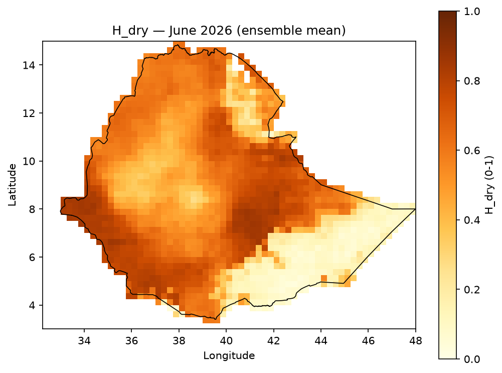
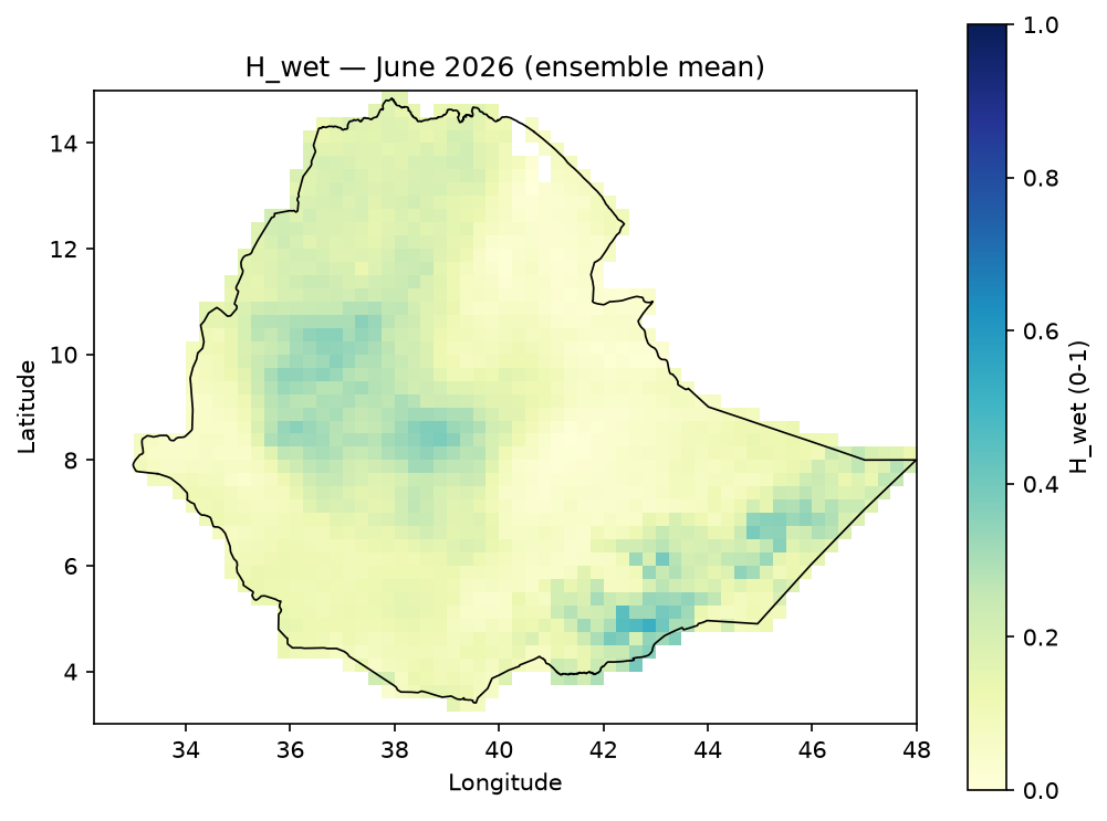
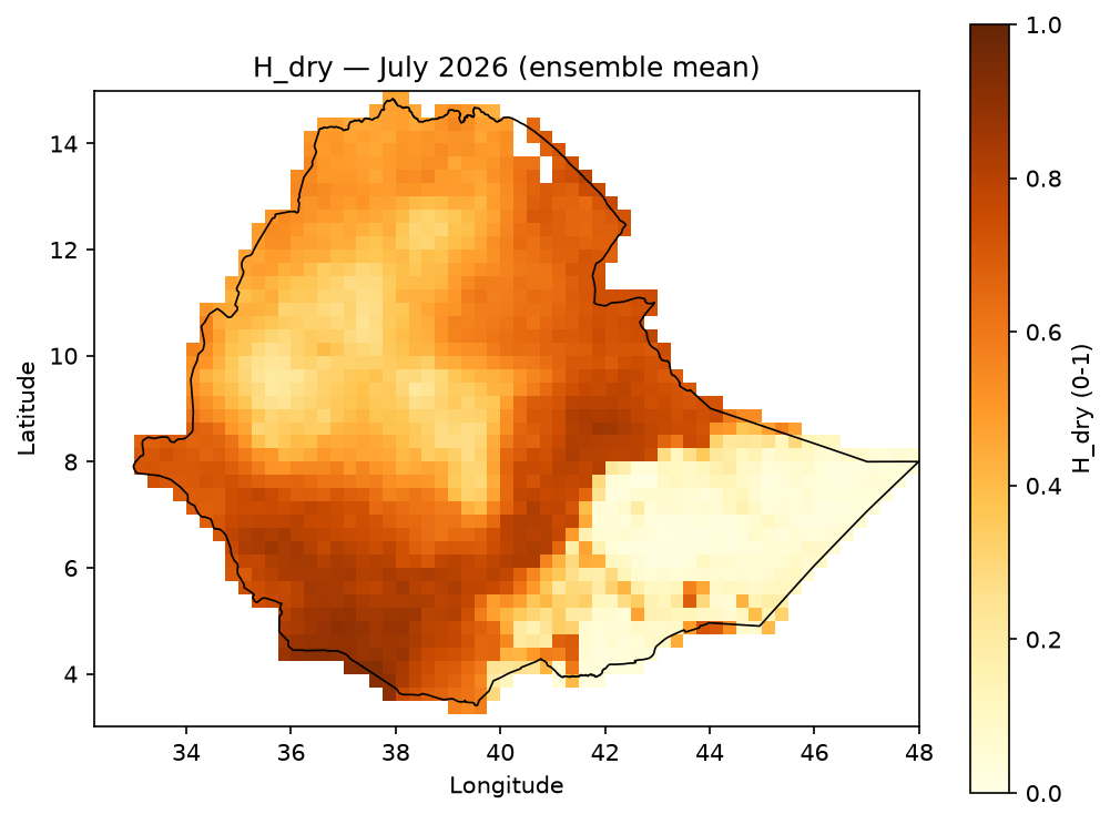
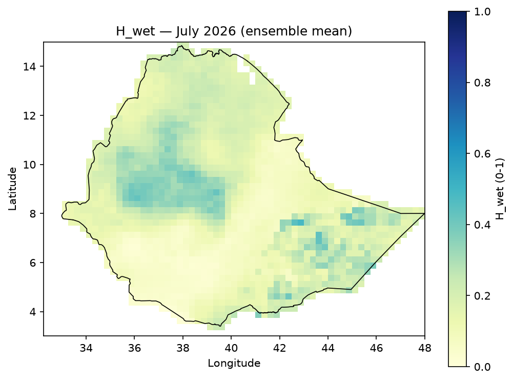
Each climate index is standardized to a 0–1 score (percentile-based for rainfall/CDD/CWD/Rx1day/Rx5day; a fixed transform for SPI), then combined with methodology-defined weights:

H_{dry} = 0.35\,S_{SPI,dry} + 0.20\,S_{rain,dry} + 0.30\,S_{CDD,dry} + 0.15\,S_{CWD,dry}

H_{wet} = 0.20\,S_{SPI,wet} + 0.20\,S_{rain,wet} + 0.20\,S_{CWD,wet} + 0.15\,S_{Rx1day,wet} + 0.25\,S_{Rx5day,wet}

Drought and wetness hazard are never averaged (opposite signals would cancel and mask a real hazard):

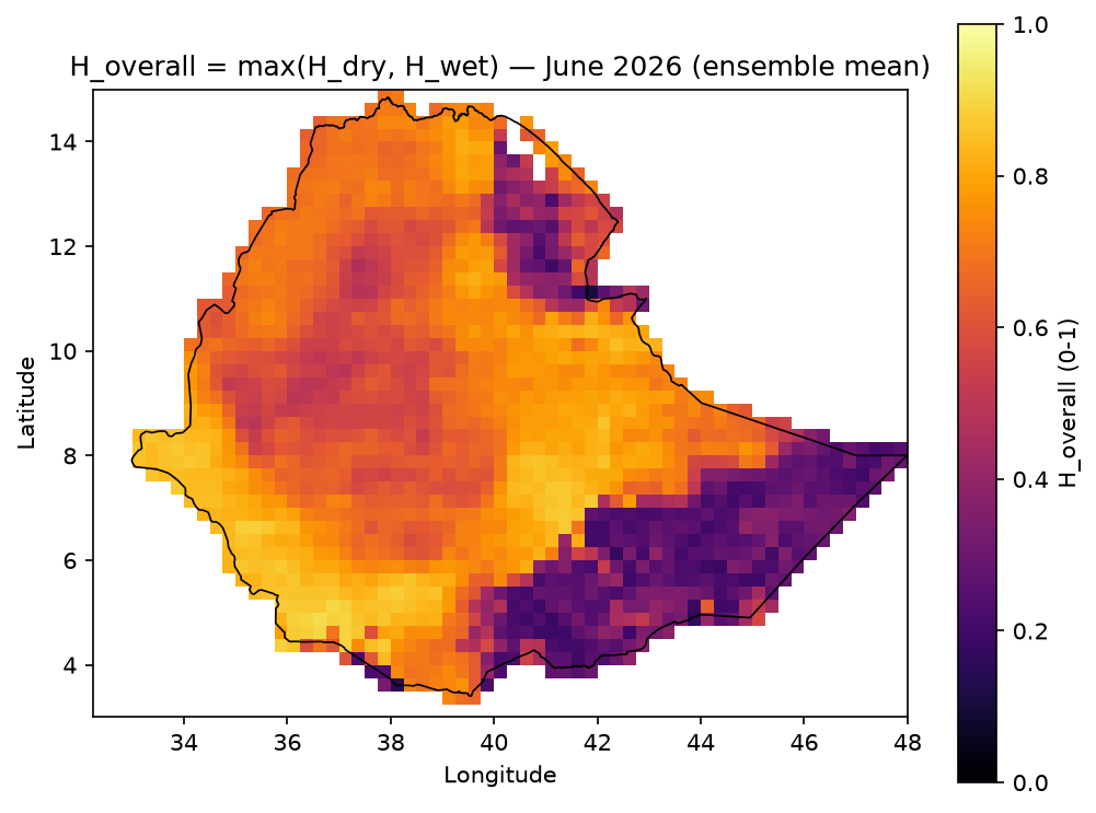
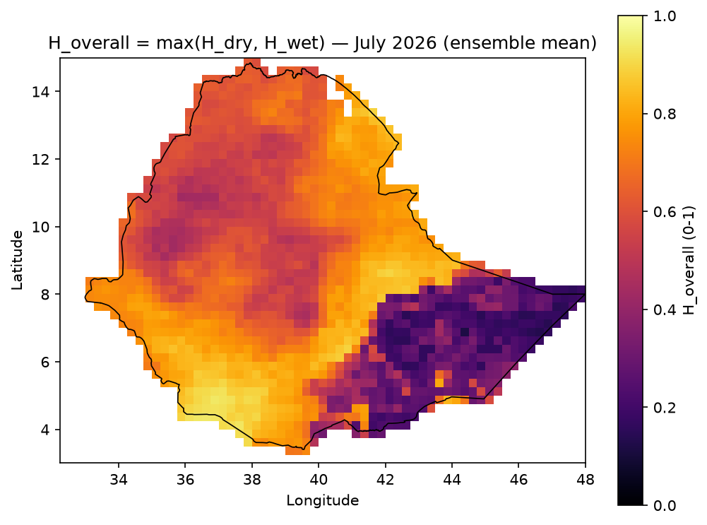
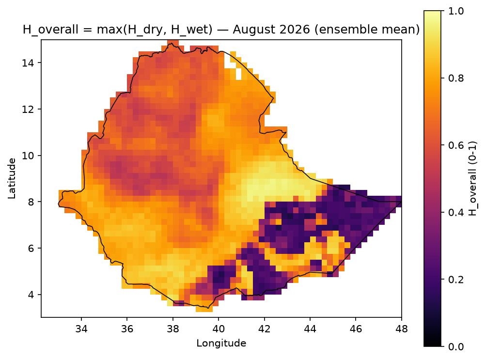
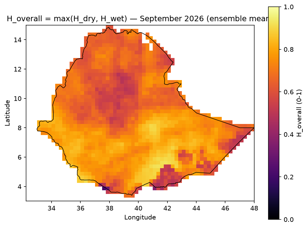
H_{overall} = \max(H_{dry}, H_{wet})

Example output — ensemble-mean H_dry / H_wet, JJAS 2026:

Monthly breakdown — H_dry / H_wet for June, July, August, September

	H_dry	H_wet
June
July
August
September

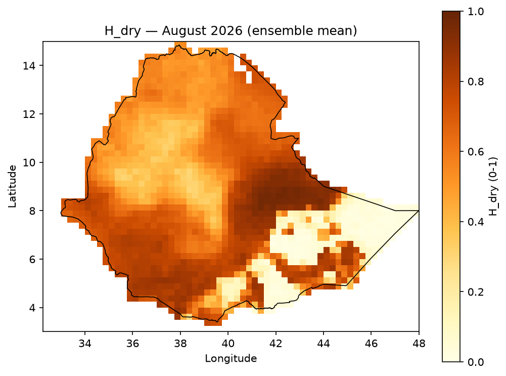
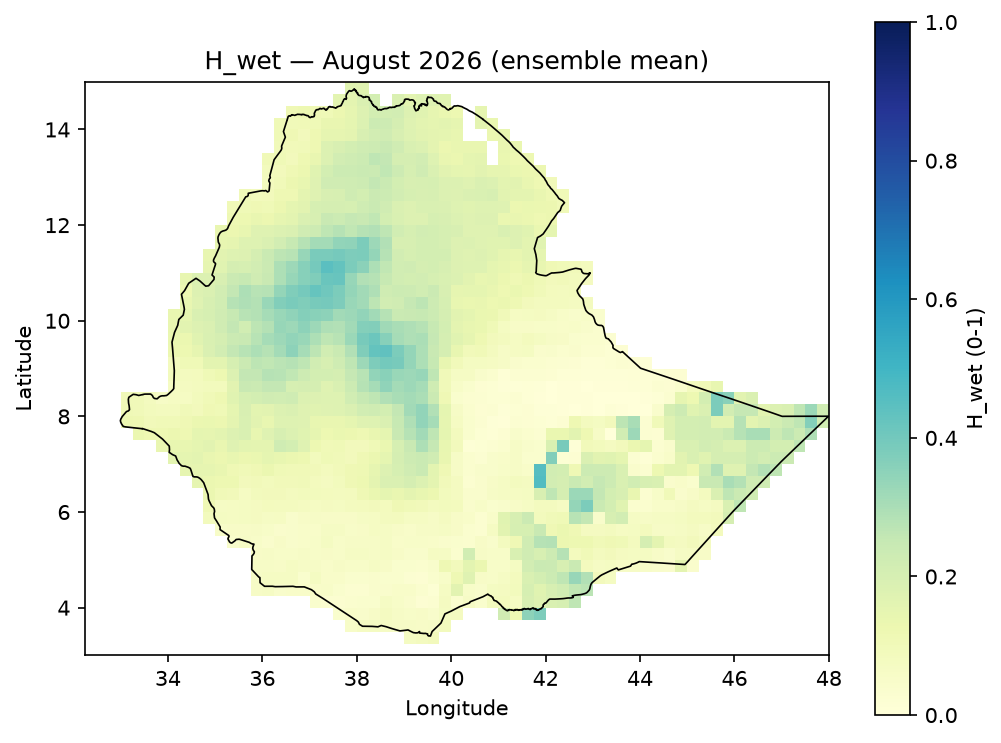
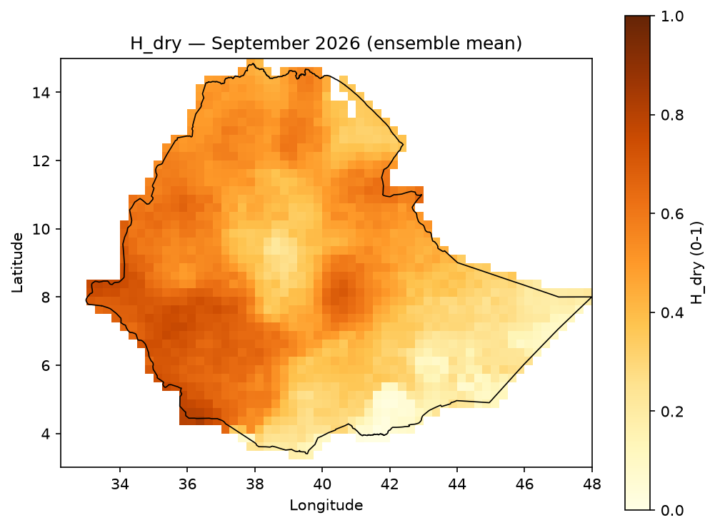
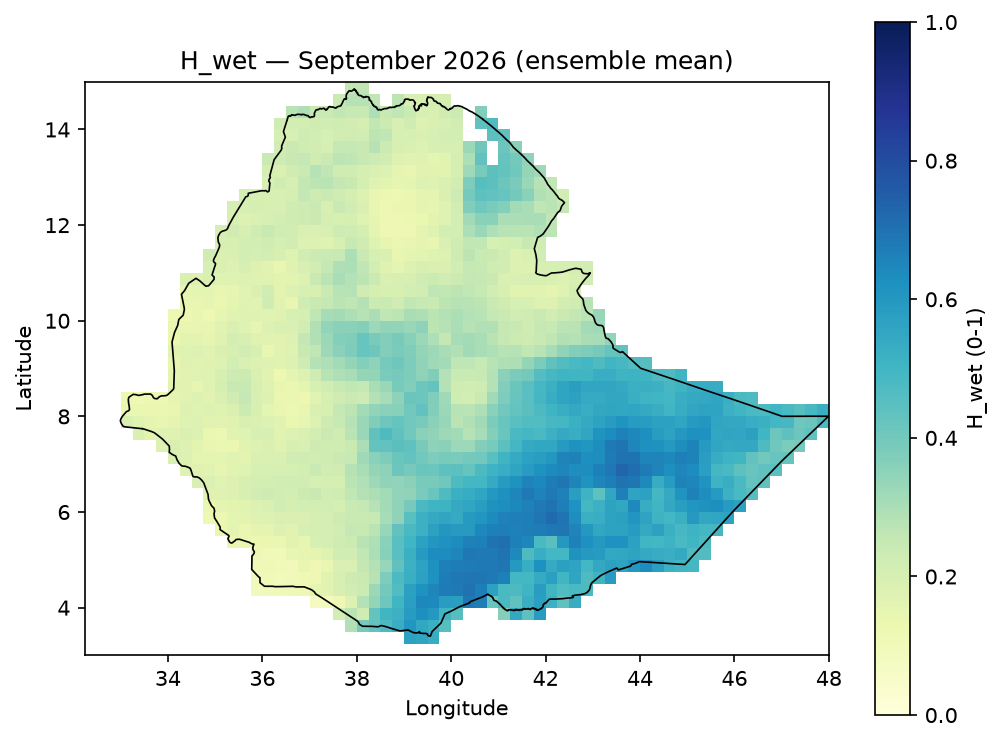
Example output — H_overall = max(H_dry, H_wet), JJAS 2026. Computed per ensemble member first, then averaged (not max of the two already-averaged maps above) — since max is convex, mean(max(H_dry, H_wet)) is always ≥ max(mean(H_dry), mean(H_wet)); verified on real JJAS data, the two differ by up to 0.35 in some cells, so the reduction order isn’t cosmetic:

[!TIP] How to read this map. H_overall answers one question only: “is at least one hazard type (drought OR excess wetness) forecast to be elevated here, on average across the ensemble?” — it does not tell you which one. In the JJAS 2026 map above, most of the country is orange/yellow (0.6–1.0) — meaning some hazard signal is elevated almost everywhere this season — except a handful of purple/dark patches (e.g. around 8–10°N, 36–39°E and a small cluster near 4°N, 41–42°E) where neither hazard is strongly forecast. To find out which hazard is driving a high value at a given cell, compare it against the H_dry/H_wet maps above, or see dominant_code in the Risk section below. A high H_overall also doesn’t imply consistent agreement across all 25 members — it can be high because most members agree on one hazard type, or because members disagree (some forecasting drought, others wetness) while each individually stays “hazardous” in its own direction; H_overall alone can’t distinguish those two very different situations.

Monthly breakdown — H_overall for June, July, August, September

June	July	August	September

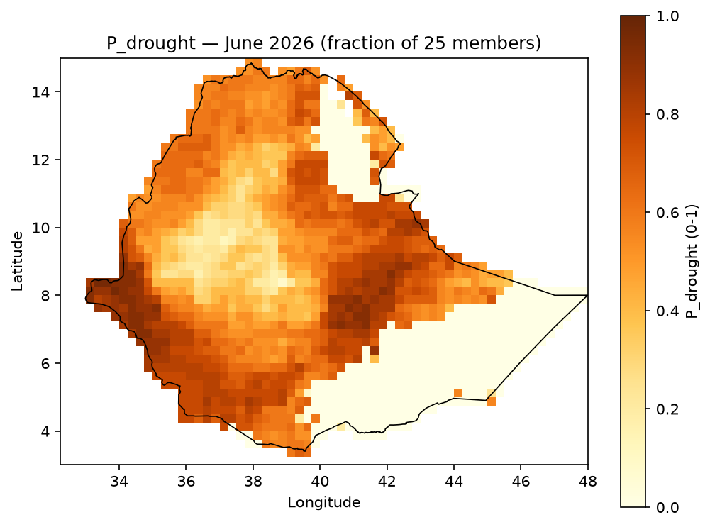
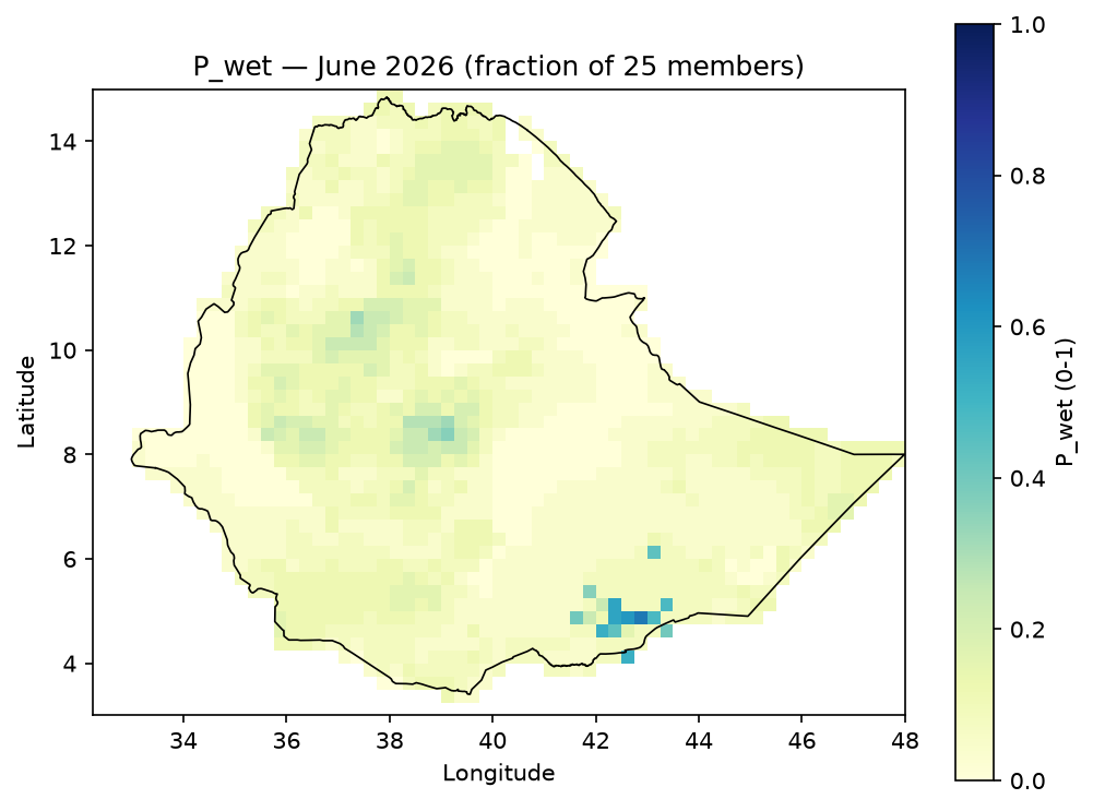
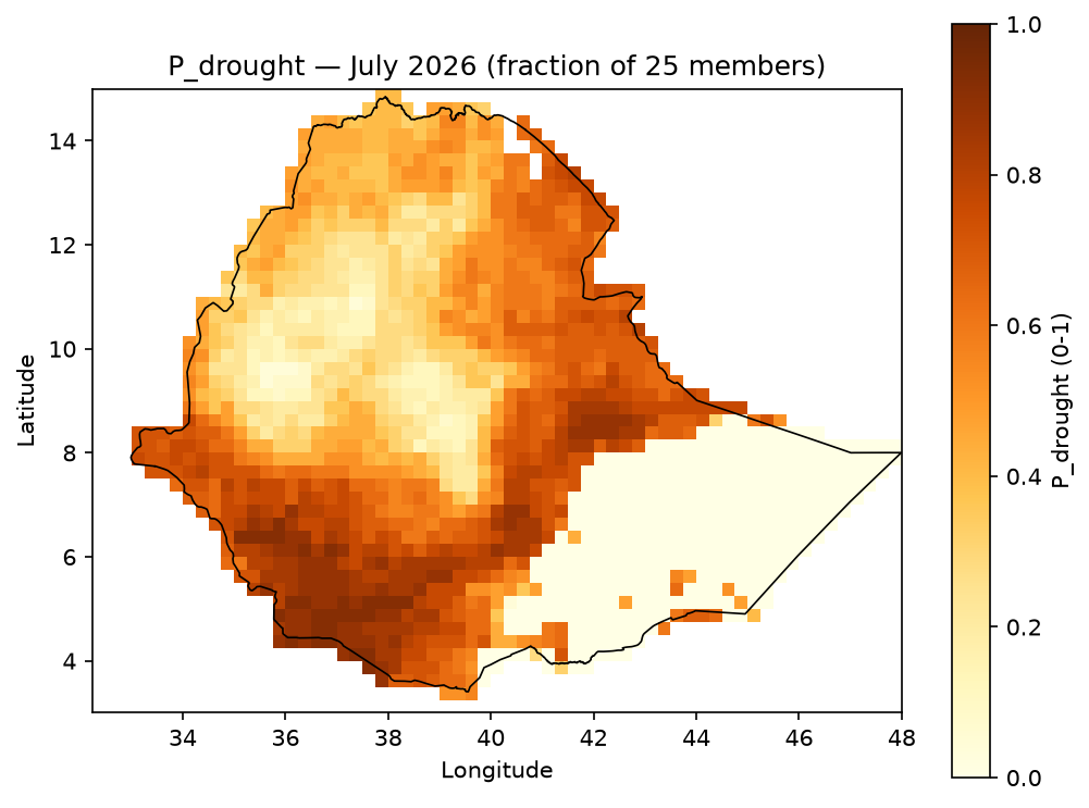
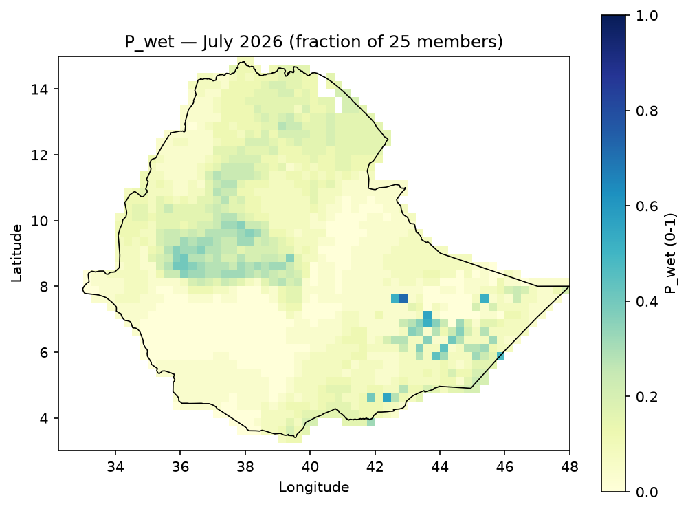
2. Probability & Severity (P, S)

Across the 25-member forecast ensemble, with a configurable high-hazard threshold (default 0.60):

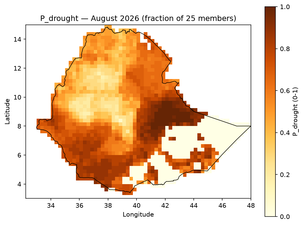
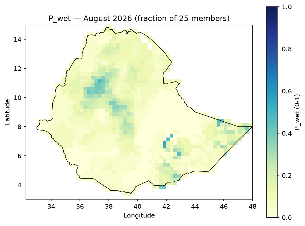
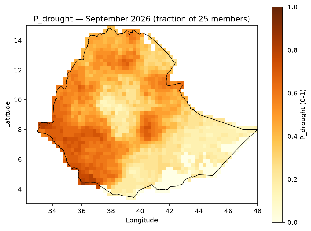
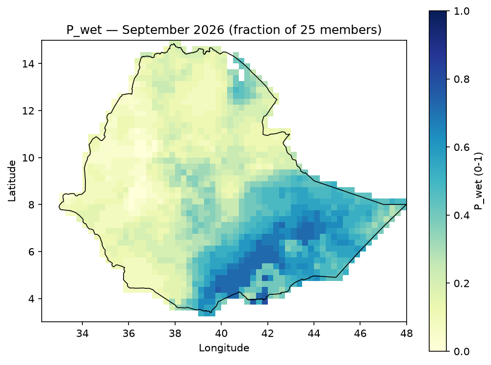
P_{drought} = \frac{\text{count}(H_{dry} \geq 0.60)}{25}, \qquad
S_{drought} = \text{mean}\big(H_{dry} \mid H_{dry} \geq 0.60\big)

(equivalently for P_wet / S_wet). P and S together operationalize hazard likelihood and conditional intensity — this is what the rest of the pipeline refers to as the hazard term.

Example output — P_drought / P_wet, JJAS 2026 (fraction of the 25-member ensemble exceeding the high-hazard threshold):

Monthly breakdown — P_drought / P_wet for June, July, August, September

	P_drought	P_wet
June
July
August
September

Example output — S_drought / S_wet, JJAS 2026 (mean hazard score among only the ensemble members that cleared the threshold — colorbar starts at 0.60, not 0, since S is undefined below that threshold rather than 0):

Monthly breakdown — S_drought / S_wet for June, July, August, September

	S_drought	S_wet
June
July
August
September

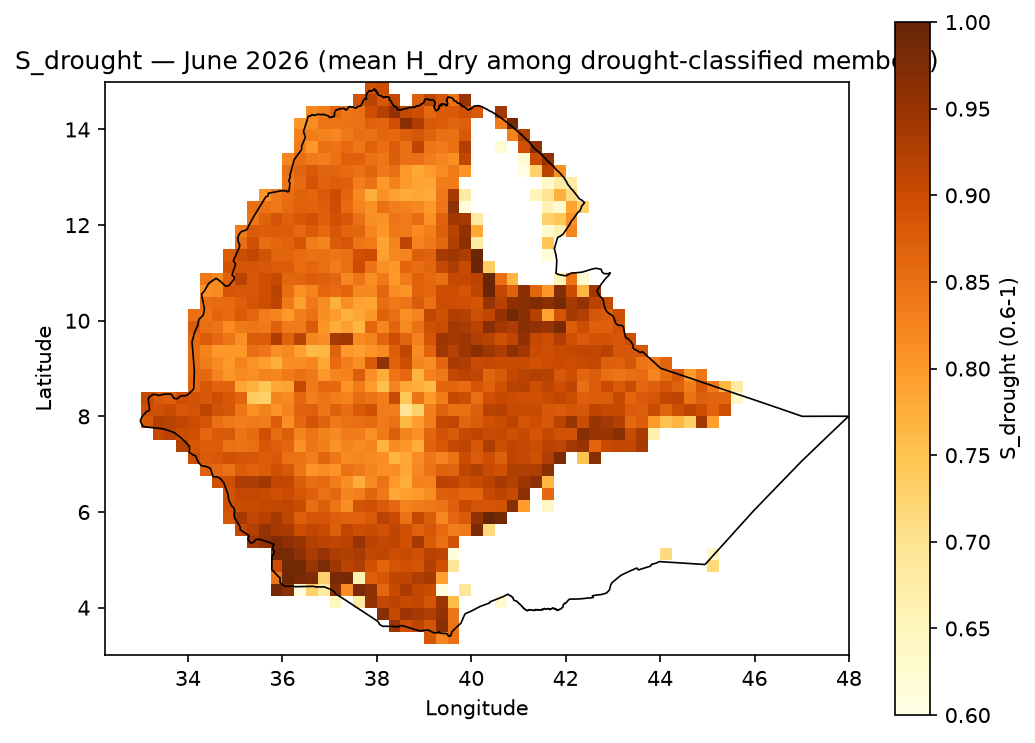
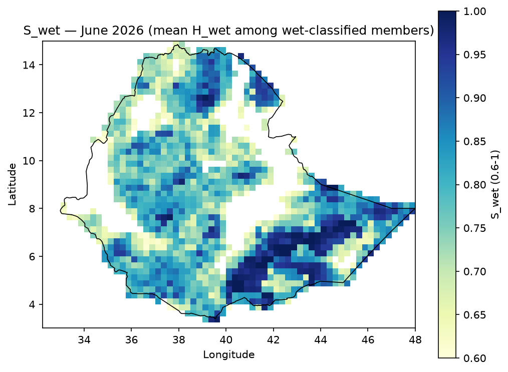
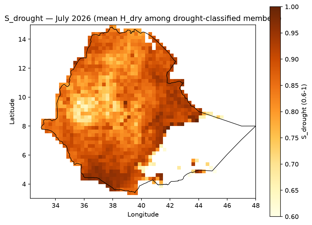
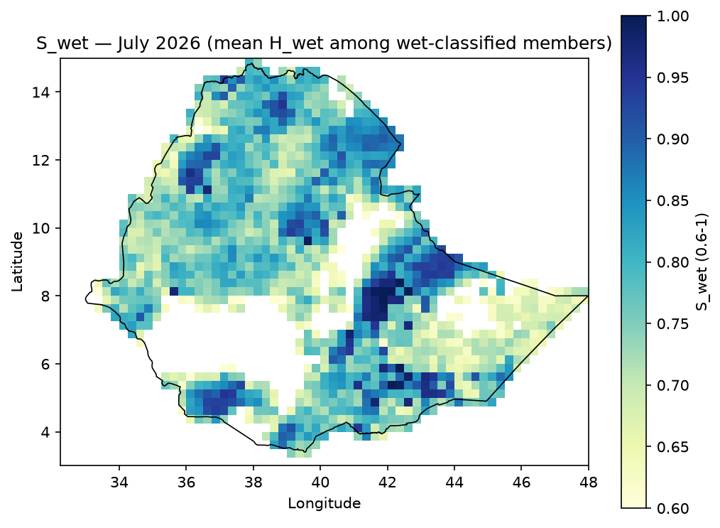
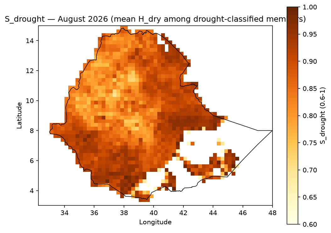
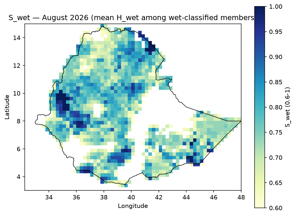
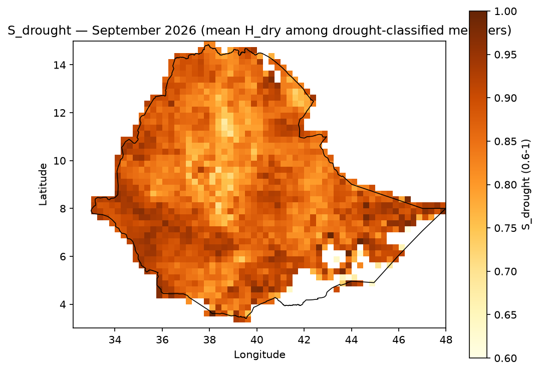
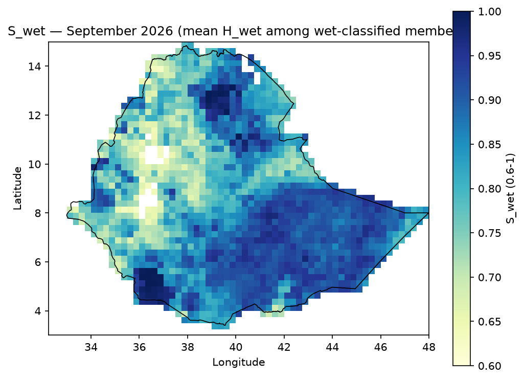
3. Exposure (E)

Absolute exposure (people, hectares, head of livestock, facility counts) is preserved per-sector — sectors are never blended into one index — and separately normalized to 0–1 via robust 5th/95th-percentile scaling:

E_{norm} = \text{clip}\left(\frac{E_{raw} - P_{5}(E)}{P_{95}(E) - P_{5}(E)},\ 0,\ 1\right)

Example output — normalized population exposure. Unlike Hazard/Probability, exposure isn’t period-dependent in this pipeline (population counts don’t vary by forecast month), so there’s a single map, not a monthly set:

4. Vulnerability (V)

Each vulnerability indicator is normalized the same way, oriented so higher always means more vulnerable (beneficial/capacity indicators are inverted), then combined:

V_{drought} = 0.60\,\text{Sensitivity}_{drought} + 0.40\,\text{AdaptiveCapacityDeficit}_{drought}

V_{wet} = 0.60\,\text{Sensitivity}_{wet} + 0.40\,\text{AdaptiveCapacityDeficit}_{wet}

Sensitivity_wet combines poverty, terrain (elevation, slope), soil drainage (clay content), and river/water-body proximity in equal proportion — see docs/data_provenance.md for why these four physical indicators were chosen.

Example output — V_drought / V_wet composite indices. Also not period-dependent (socioeconomic/terrain vulnerability doesn’t change month to month), so one map each:

5. Risk (R)

The full composition, conceptually Risk = Hazard × Exposure × Vulnerability, is implemented per hazard type as:

R_{drought} = 100 \times P_{drought} \times S_{drought} \times E_{norm} \times V_{drought}

R_{wet} = 100 \times P_{wet} \times S_{wet} \times E_{norm} \times V_{wet}

R_{dominant} = \max(R_{drought}, R_{wet})

R is a relative 0–100 risk score, not a probability percentage, classified into five bands:

Range	Class	Code
0–19.9	Very low	0
20–39.9	Low	1
40–59.9	Moderate	2
60–79.9	High	3
80–100	Very high	4

Example output — R_drought / R_wet, population sector, JJAS 2026 (the two hazard-specific risk scores that feed everything below):

Example output — R_dominant = max(R_drought, R_wet), population sector, JJAS 2026:

[!TIP] How to read this map, and why it looks so different from H_overall above. H_overall was orange/yellow (elevated) across nearly the entire country; R_dominant here is pale/near-zero almost everywhere except a few concentrated hotspots (e.g. ~9°N, 42–44°E and a cluster around 6–8°N, 36–40°E). That’s not a bug — it’s the whole point of the Hazard × Exposure × Vulnerability framework. R_dominant isn’t hazard alone: it’s hazard gated by whether P/S cross the significance threshold, then multiplied by both normalized exposure and vulnerability. A cell can have high H_overall (a real, forecast-elevated hazard) and still land near-zero R_dominant if that cell has little population exposure there, or low population-sector vulnerability — hazard without anything exposed and vulnerable to it isn’t risk. The bright spots on this map are exactly where elevated hazard coincides with people who are both present and vulnerable — read together with E_population and V_drought/V_wet above to see why a given hotspot is a hotspot (high exposure there? high vulnerability? both?).

Alongside risk_class, every batch run also writes a dominant_code layer (dominant_risk_code() in risk/risk.py). It’s easy to assume this is just argmax(R_drought, R_wet) (whichever is numerically larger) — it isn’t. Each of R_drought/R_wet is independently tested against the “Very low” band’s ceiling (19.9) before being compared to the other:

Code	Label	Condition
0	None / insignificant	neither R_drought nor R_wet exceeds 19.9
1	Drought-dominated	only R_drought exceeds 19.9
2	Wet-dominated	only R_wet exceeds 19.9
3	Mixed / compound	both exceed 19.9

This matters because a plain argmax always picks a winner, even between two barely-nonzero values — it would mislabel every genuinely low-risk cell as “drought” or “wet” dominant. In the real population/JJAS output, 1,398 of 1,479 valid cells (94.5%) are code 0; a naive argmax would have force-assigned all of them to a hazard type that isn’t actually significant there. dominant_code reuses the same 0=none / 1=drought / 2=wet / 3=mixed numbering as hazard.dominant_hazard_code (methodology.md’s convention for keeping the two layers consistent), but it’s computed from R, not H — don’t assume the two rasters have identical values just because they share a coding scheme. Note this is a categorical layer (a hazard type, not a magnitude) — the map below uses a discrete color per code rather than a continuous scale, since “Wet”=2 isn’t “twice” “Drought”=1:

Example output — risk_class, the five-band classification of R_dominant, population sector, JJAS 2026:

Why population, and what’s actually in outputs/risk/

R = 100 × P × S × E × V is computed separately per exposure sector — a hospital-poor area and a hospital-rich area have identical Hazard/Probability/Vulnerability but very different infrastructure-sector risk. Nothing here is limited to population; the full batch run (python scripts/hydroclim_risk_cli.py generate-risk, see scripts/03_generate_risk_maps.py) already writes outputs/risk/ in full:

outputs/risk/ethiopia_{period}_{init_date}_{sector}_{product}.tif

Axis	Values	Count
period	June, July, August, September, JJAS	5
sector	population, cropland_total, cropland_irrigated, cropland_rainfed, livestock_cattle, buildings, roads, healthsites, built_up	9
product	r_drought, r_wet, r_dominant, dominant_code, risk_class	5

5 × 9 × 5 = 225 GeoTIFFs, all already generated and QC-passed. population is used for the two README images above purely as one illustrative, easy-to-interpret sector so this document shows two maps instead of 45 (9 sectors × 5 products for JJAS alone) — it’s a documentation choice, not a pipeline limitation. Swap SECTOR in scripts/04_generate_doc_images.py / scripts/05_generate_stage_geotiffs.py to regenerate the same example set for any other sector, or read any of the 225 files directly — e.g. outputs/risk/ethiopia_JJAS_2026-05-01_healthsites_risk_class.tif for health-facility risk instead of population risk.

[!NOTE] All 43 PNGs across the sections above (Hazard × 5 periods × {H_dry, H_wet, H_overall}, Probability & Severity × 5 periods × {P_drought, P_wet, S_drought, S_wet}, Exposure ×1, Vulnerability ×2, Risk × {r_drought, r_wet, r_dominant, dominant_code, risk_class} = 5) are generated by scripts/04_generate_doc_images.py from this pipeline’s real output — not mockups. The GeoTIFF counterpart of every image here is written by scripts/05_generate_stage_geotiffs.py to outputs/hazard/, outputs/probability/, outputs/exposure/, outputs/vulnerability/, and outputs/risk/ respectively (not tracked in git — regenerate on demand). Re-run both scripts after any pipeline change to refresh these images/files.

Pipeline Architecture

┌──────────────────────────────────────────────────────────────────────────┐
│                              RAW DATA SOURCES                            │
│  Ensemble NetCDF forecasts  │  Exposure rasters/vectors  │  Vulnerability │
│  (bias-corrected/*.nc)      │  (WorldPop, WorldCover...)  │  (SoilGrids,  │
│                              │                              │  ETOPO...)  │
└───────────────┬───────────────────────┬──────────────────────┬──────────┘
                │                       │                      │
                ▼                       ▼                      ▼
        ┌───────────────┐     ┌──────────────────┐   ┌──────────────────┐
        │  INGESTION     │     │  ACQUISITION      │   │  ACQUISITION      │
        │  netcdf.py     │     │  (11 modules,      │   │  (vulnerability    │
        │  members.py    │     │   src/.../         │   │   sub-set of the   │
        │  geotiff.py    │     │   acquisition/)     │   │   same modules)    │
        │  boundaries.py │     │  download → warp →  │   │  download → warp → │
        │                │     │  resample to grid    │   │  resample to grid  │
        └───────┬────────┘     └──────────┬───────────┘   └──────────┬────────┘
                │                          │                          │
                ▼                          ▼                          ▼
        ┌───────────────┐        ┌──────────────────┐       ┌──────────────────┐
        │  HAZARD        │        │  EXPOSURE         │       │  VULNERABILITY    │
        │  standardize    │        │  per-sector         │       │  sensitivity +     │
        │  H_dry / H_wet  │        │  absolute + 0-1      │       │  adaptive-capacity │
        │  (hazard/)      │        │  normalized           │       │  deficit (vuln-    │
        │                │        │  (exposure/)          │       │  erability/)        │
        └───────┬────────┘        └──────────┬───────────┘       └──────────┬────────┘
                │                             │                             │
                ▼                             │                             │
        ┌───────────────┐                    │                             │
        │  PROBABILITY   │                    │                             │
        │  P_drought/wet │                    │                             │
        │  S_drought/wet │                    │                             │
        │  (probability/)│                    │                             │
        └───────┬────────┘                    │                             │
                │                             │                             │
                └──────────────┬──────────────┴──────────────┬──────────────┘
                               ▼                              ▼
                    ┌────────────────────────────────────────────────┐
                    │                   RISK                          │
                    │  R = 100 × P × S × E × V   (risk/pipeline.py)   │
                    │  R_dominant, dominant_code, risk_class           │
                    └───────────────────────┬──────────────────────────┘
                                            ▼
                    ┌────────────────────────────────────────────────┐
                    │        VALIDATION  →  RASTER EXPORT             │
                    │  grid alignment, Inf/constant checks             │
                    │  (validation/)        GeoTIFF + PNG quicklook    │
                    │                        (export/)                 │
                    └────────────────────────────────────────────────┘

Orchestrated end-to-end by scripts/03_generate_risk_maps.py (and equivalently, hydroclim_risk generate-risk): vulnerability is computed once (static across periods), hazard/probability once per period, then combined with each exposure sector — keeping a full 5-period × 9-sector batch to a few seconds.

Installation & Setup

Requirements: Python 3.11+ (developed and tested against 3.11.9), and a GDAL-capable environment (via rasterio/geopandas’s binary wheels — no separate system GDAL install is required on most platforms).

# 1. Clone the repository
git clone https://github.com/YonSci/hydroclimatic-risk-mapping.git
cd hydroclimatic-risk-mapping

# 2. Create and activate a virtual environment
python -m venv .venv
source .venv/bin/activate        # Linux/macOS
.venv\Scripts\activate           # Windows

# 3. Install dependencies
pip install -r requirements.txt

# 4. Verify the environment
python scripts/00_check_environment.py

[!IMPORTANT] This project has no editable package install — every entry point (scripts and the CLI wrapper) manually inserts src/ onto sys.path. Run scripts and the CLI wrapper from the repository root as shown below rather than pip install -e ..

For a fully pinned, reproducible environment, requirements-lock.txt captures exact versions from a known-working install:

pip install -r requirements-lock.txt

Run the test suite to confirm the install is healthy:

pytest -q
# 242 passed

CLI & Module Usage

Command-line interface

# Verify every required package imports correctly
python scripts/hydroclim_risk_cli.py check-env

# Download and resample all exposure/vulnerability datasets (or a subset)
python scripts/hydroclim_risk_cli.py download-data
python scripts/hydroclim_risk_cli.py download-data --only population,livestock,terrain

# Compute and write R_drought / R_wet / R_dominant / risk_class GeoTIFFs
python scripts/hydroclim_risk_cli.py generate-risk
python scripts/hydroclim_risk_cli.py generate-risk --periods June,JJAS --sectors population

# QC a directory of GeoTIFF outputs (Inf values, constant/zero-variance rasters)
python scripts/hydroclim_risk_cli.py validate --directory outputs/risk

Equivalently, as a module (identical behavior — the wrapper only adds src/ to sys.path):

python -m hydroclim_risk.cli generate-risk --periods JJAS

Running individual pipeline stages as modules

import sys
sys.path.insert(0, "src")

from hydroclim_risk.config import load_data_config
from hydroclim_risk.risk.pipeline import compute_hazard_and_probability_for_period
from hydroclim_risk.exposure import compute_exposure_layer
from hydroclim_risk.vulnerability import compute_v_drought, compute_v_wet
from hydroclim_risk.risk.risk import compute_risk, classify_risk

domain_cfg = load_data_config()

# Hazard + ensemble probability/severity for one period
hazard_prob = compute_hazard_and_probability_for_period("JJAS")

# Static vulnerability composites (shared across all periods/sectors)
v_drought = compute_v_drought(domain_cfg=domain_cfg)
v_wet = compute_v_wet(domain_cfg=domain_cfg)

# One exposure sector
population = compute_exposure_layer("population", domain_cfg=domain_cfg)

# Final risk
r_drought = compute_risk(
    hazard_prob["p_drought"], hazard_prob["s_drought"],
    population.normalized, v_drought,
)
risk_class = classify_risk(r_drought)

Standalone demo (no real data required)

python examples/synthetic_demo.py

Runs the full hazard → probability → exposure → vulnerability → risk chain against synthetic in-memory data, useful for smoke-testing an install without downloading anything.

Project Structure

hydroclimatic-risk-mapping/
├── .github/workflows/ci.yml         # GitHub Actions: pytest (blocking) + ruff (advisory)
├── config/                          # Every threshold/weight/path — single source of truth
│   ├── data.yaml                    #   domain grid, ensemble slicing, file paths
│   ├── periods.yaml                 #   reference climatology, assessment period, labels
│   ├── thresholds.yaml              #   hazard threshold, SPI cap, risk-class bands
│   ├── weights.yaml                 #   H_dry/H_wet/V_drought/V_wet weights
│   ├── standardization.yaml         #   per-indicator standardization decisions
│   ├── exposure_data.yaml           #   exposure/vulnerability acquisition registry
│   ├── exposure_indicators.yaml     #   exposure layer registry (9 sectors)
│   └── vulnerability_indicators.yaml#   vulnerability indicator registry
│
├── src/hydroclim_risk/
│   ├── ingestion/                   # NetCDF, GeoTIFF, per-member, boundary readers
│   ├── acquisition/                 # 13 external dataset downloader/resampler modules
│   ├── hazard/                      # Standardization + H_dry/H_wet scoring
│   ├── probability/                 # Ensemble P_drought/P_wet, S_drought/S_wet
│   ├── exposure/                    # Per-sector exposure normalization
│   ├── vulnerability/               # V_drought/V_wet composite indices
│   ├── risk/                        # R = 100×P×S×E×V, classification, orchestration
│   ├── validation/                  # Grid-alignment + QC report generation
│   ├── export/                      # GeoTIFF → PNG quicklook rendering
│   ├── layers.py                    # Shared normalization/gap-fill/masking helpers
│   ├── scoring.py                   # Shared weighted-sum combination logic
│   ├── config.py                    # YAML config loader + validation
│   └── cli.py                       # Typer CLI (check-env/download-data/generate-risk/validate)
│
├── scripts/                         # Standalone entry points (no editable install needed)
│   ├── 00_check_environment.py
│   ├── 02_download_exposure_vulnerability_data.py
│   ├── 03_generate_risk_maps.py
│   ├── 04_generate_doc_images.py    # Regenerates docs/images/ example maps from real output
│   └── hydroclim_risk_cli.py
│
├── examples/
│   └── synthetic_demo.py            # Full pipeline against synthetic data, no downloads
│
├── tests/                           # 242 tests — real-data smoke tests + synthetic unit tests
│
├── docs/
│   ├── methodology.md               # Full formula reference
│   ├── data_provenance.md           # Every dataset: source, license, citation, caveats
│   └── images/                      # Example output maps embedded in this README
│
├── boundaries/                      # Ethiopia admin0-3 shapefiles (bundled, not downloaded)
├── bias-corrected/                  # Source ensemble NetCDFs (not tracked in git — see below)
├── chrips_historical/               # CHIRPS observational NetCDF (not tracked in git)
├── data/                            # Raw downloaded exposure/vulnerability cache (not tracked)
├── outputs/                         # Generated GeoTIFFs, PNGs, QC tables (not tracked)
│
├── requirements.txt                 # Direct dependencies
├── requirements-lock.txt            # Fully pinned, reproducible install
├── pyproject.toml                   # pytest + ruff configuration
├── .gitignore
├── LICENSE                          # MIT (code only — see License & Citation)
└── README.md

[!NOTE] bias-corrected/, chrips_historical/, data/, and outputs/ hold large binary climate/geospatial data and generated results — excluded via .gitignore and never pushed. boundaries/ (~22 MB of shapefiles) is intentionally tracked: it’s a small, bundled asset the test suite and pipeline both read directly, not a download. Obtain the excluded data per docs/data_provenance.md, or regenerate exposure/vulnerability layers via download-data (see CLI & Module Usage).

License & Citation

This project’s code is licensed under the MIT License — see LICENSE for the full text.

[!IMPORTANT] The MIT license covers this repository’s source code only. It does not relicense the third-party datasets the pipeline downloads and redistributes derived products from — several of those (OSM/Geofabrik, Meta RWI) carry their own share-alike or attribution requirements (ODbL, CC-BY 4.0) that remain binding on any output you publish. See below and docs/data_provenance.md for the full per-source terms.

Upstream data attribution. This pipeline redistributes derived products from several third-party datasets, each requiring attribution per their own license (CC-BY 4.0 or ODbL) — do not drop these citations when publishing outputs. Full citations for every source are in docs/data_provenance.md, including:

• WorldPop (population), ESA WorldCover (cropland), FAO GLW4 (livestock), JRC GHSL (built-up surface), CGIAR-CSI (aridity index), FAO/Bonn GMIA v5 (irrigation), Falchetta et al./IIASA (GDESSA electrification access), NOAA NCEI (ETOPO 2022), ISRIC (SoilGrids 2.0)

• © OpenStreetMap contributors, via Geofabrik and the Global Healthsites Mapping Project (ODbL — share-alike attribution required)

• © Meta Platforms, Inc. (Relative Wealth Index, via Data for Good)

Citing this repository. Until a formal citation file (CITATION.cff) is added, cite as:

Ethiopia Hydroclimatic Risk Mapping Pipeline. YonSci, 2026.
https://github.com/YonSci/hydroclimatic-risk-mapping