Mapping Geographical Data with Basemap Python Package
Basemap is a matplotlib extension used to visualize and create geographical maps in python. The main purpose of this tutorial is to provide basic information on how to plot and visualize geographical data with the help of Basemap package. If you need further information on basemap, please visit basemap page.
- Installing Basemap package
- Adding vector layers to a map
- Projection, bounding box, & resolution
- Plotting a specific region
- Background relief maps
- Plotting netCDF data using Basemap
Installing Basemap package
1) Start an Ubuntu terminal or an Anaconda prompt
2) Add a new environment variable named basemap_stable
conda create --name basemap_stable3) Activate the basemap_stable environment:
conda activate basemap_stable4) Install basemap package and it’s :
conda install -c anaconda basemap5) View a list of python dependencies by typing conda list
conda list6) Now open your favorite Python Notebook or IDE in the active conda environment, In my case, i used jupyter notebook
7) Finally, import the Basemap and Matplotlib libraries:
from mpl_toolkits.basemap import Basemap
import matplotlib.pyplot as plt
Adding vector layers to a map
Coastlines
- First, let’s initialize a map with
Basemap()function - Then, use the
drawcoastlines()function to add coastlines on the map
fig = plt.figure(figsize = (12,12))
m = Basemap()
m.drawcoastlines()
plt.title("Coastlines", fontsize=20)
plt.show()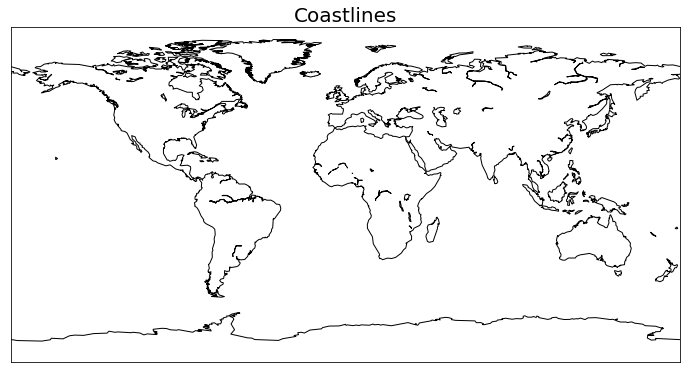
The drawcoastlines function has the following main arguments:
- linewidth: 1.0, 2.0, 3.0…
- linestyle: solid, dashed…
- color: black, red…
Let’s apply some changes to the coastlines
fig = plt.figure(figsize = (12,12))
m = Basemap()
m.drawcoastlines(linewidth=1.0, linestyle='dashed', color='red')
plt.title("Coastlines", fontsize=20)
plt.show()
Countries
Use the drawcountries() function to add countries on the map
fig = plt.figure(figsize = (12,12))
m = Basemap()
m.drawcoastlines(linewidth=1.0, linestyle='solid', color='black')
m.drawcountries()
plt.title("Country boundaries", fontsize=20)
plt.show()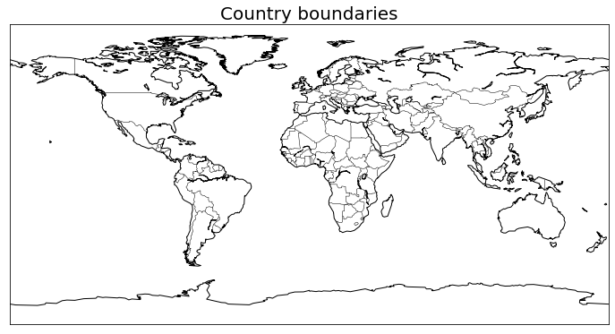
The drawcountries() function uses similar arguments like drawcountries() as shown below:
fig = plt.figure(figsize = (12,12))
m = Basemap()
m.drawcoastlines(linewidth=1.0, linestyle='solid', color='black')
m.drawcountries(linewidth=1.0, linestyle='solid', color='k')
plt.title("Country boundaries", fontsize=20)
plt.show()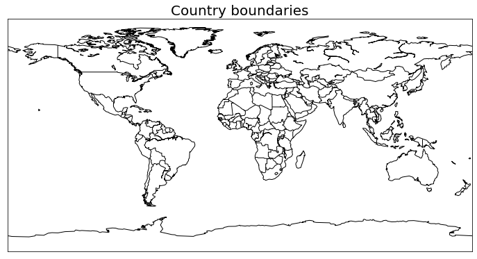
Draw major rivers
Use the
drawrivers()function to add major rivers on the mapThe
drawrivers()function can takelinewidth,linestyle,colorarguments
fig = plt.figure(figsize = (12,12))
m = Basemap()
m.drawcoastlines(linewidth=1.0, linestyle='solid', color='black')
m.drawcountries(linewidth=1.0, linestyle='solid', color='k')
m.drawrivers(linewidth=0.5, linestyle='solid', color='#0000ff')
plt.title("Major rivers", fontsize=20)
plt.show()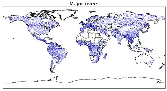
Fill continents
- This function is used to draw color filled continents
- Use
fillcontinents()function to fill continents
fig = plt.figure(figsize = (12,12))
m = Basemap()
m.drawcoastlines(linewidth=1.0, linestyle='solid', color='black')
m.drawcountries(linewidth=1.0, linestyle='solid', color='k')
m.fillcontinents()
plt.title("Color filled continents", fontsize=20)
plt.show()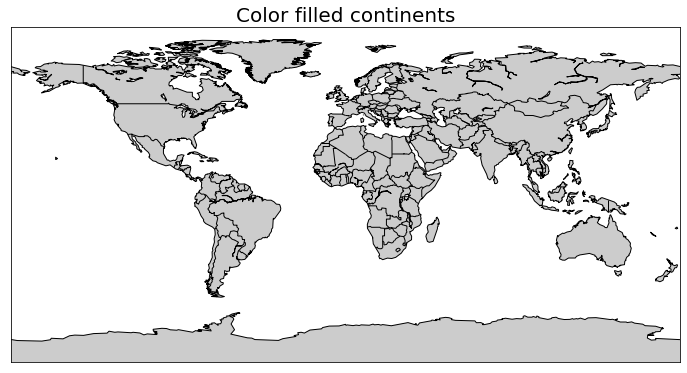
The fillcontinents() function can take the following arguments:
color: fills continents (default gray)lake_color: fills inland lakesalpha: sets transparency for continents
fig = plt.figure(figsize = (12,12))
m = Basemap()
m.drawcoastlines(linewidth=1.0, linestyle='solid', color='black')
m.drawcountries(linewidth=1.0, linestyle='solid', color='k')
m.fillcontinents(color='coral',lake_color='aqua', alpha=0.9)
plt.title("Color filled continents", fontsize=20)
plt.show()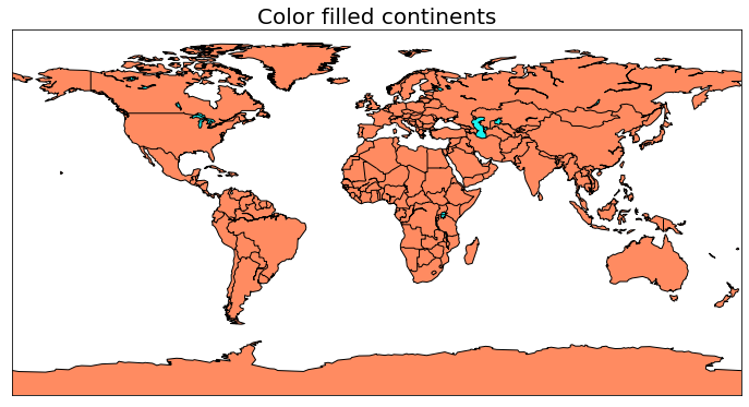
e) Draw map boundary
The
drawmapboundary()function is used to draw the earth boundary on the mapThe
drawmapboundary()function can take the following arguments:linewidth: sets line width for boundary line (default: 1)color: sets the color of the boundary line (default: black)fill_color: fills the map background region
fig = plt.figure(figsize = (12,12))
m = Basemap()
m.drawcoastlines(linewidth=1.0, linestyle='solid', color='black')
m.drawcountries(linewidth=1.0, linestyle='solid', color='k')
m.fillcontinents(color='coral',lake_color='aqua')
m.drawmapboundary(color='b', linewidth=2.0, fill_color='aqua')
plt.title("Filled map boundary", fontsize=20)
plt.show()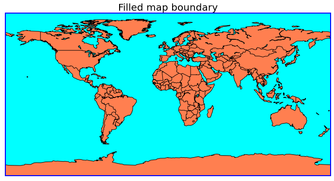
Draw and label longitude lines
- The
drawmeridians()function is used to draw & label meridians/longitude lines The
drawmeridians()function can take the following arguments:List of longitude values created with
range()for integer values &np.arange()for floats valuescolor: sets the color of the line longitude lines (default: black)textcolor: sets the color of labels (default: black)linewidth: sets the line width for the longitude linesdashes: sets the dash pattern for the longitude lines (default: [1,1])labels: sets the label’s position with four values [0,0,0,0] representing left, right, top, & bottom. Change these values to 1 where you want the labels to appear
fig = plt.figure(figsize = (12,12))
m = Basemap()
m.drawcoastlines(linewidth=1.0, linestyle='solid', color='black')
m.drawcountries(linewidth=1.0, linestyle='solid', color='k')
m.fillcontinents(color='coral',lake_color='aqua')
m.drawmeridians(range(0, 360, 20), color='k', linewidth=1.0, dashes=[4, 4], labels=[0, 0, 1, 1])
plt.title("Longitude lines", fontsize=20, pad=30)
plt.show()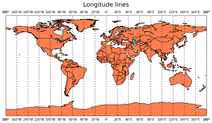
Draw and label latitude lines
The
drawparallels()function is used to draw & label parallels/latitude linesThe
drawparallels()function uses similar arguments likedrawmeridians()
fig = plt.figure(figsize = (12,12))
m = Basemap()
m.drawcoastlines(linewidth=1.0, linestyle='solid', color='black')
m.drawcountries(linewidth=1.0, linestyle='solid', color='k')
m.fillcontinents(color='coral',lake_color='aqua')
m.drawparallels(range(-90, 100, 10), color='k', linewidth=1.0, dashes=[4, 4], labels=[1, 1, 0, 0])
plt.title("Latitude lines", fontsize=20)
plt.show()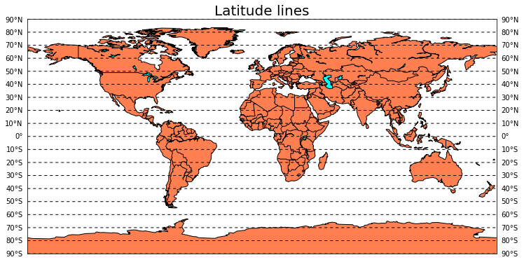
Let’s put the drawmeridians and drawparallels functions together
fig = plt.figure(figsize = (12,12))
m = Basemap()
m.drawcoastlines(linewidth=1.0, linestyle='solid', color='black')
m.drawcountries(linewidth=1.0, linestyle='solid', color='k')
m.fillcontinents(color='coral',lake_color='aqua')
m.drawmeridians(range(0, 360, 20), color='k', linewidth=1.0, dashes=[4, 4], labels=[0, 0, 0, 1])
m.drawparallels(range(-90, 100, 10), color='k', linewidth=1.0, dashes=[4, 4], labels=[1, 0, 0, 0])
plt.ylabel("Latitude", fontsize=15, labelpad=35)
plt.xlabel("Longitude", fontsize=15, labelpad=20)
plt.show()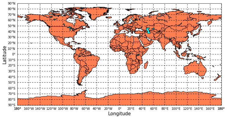
Projection, bounding box, & resolution
The Basemap() function is used to set projection, bounding box, & resolution of a map
Map projection:
Inside the
Basemap()function, theprojection="argument can take several pre-defined projections listed in the table below or visit this site to get more information.To specify the desired projection, use the general syntax shown below:
m = Basemap(projection='aeqd')
m = Basemap(projection='cyl')
| Projection name | Basemap syntax | Projection name | Basemap syntax | |
|---|---|---|---|---|
| Equidistant Conic | eqdc | Cylindrical Equal Area | cea | |
| Miller Cylindrical | mill | McBryde-Thomas Flat-Polar Quartic | mbtfpq | |
| Mercator | merc | Azimuthal Equidistant | aeqd | |
| Stereographic | stere | Sinusoidal | sinu | |
| Polyconic | poly | Rotated Pole | rotpole | |
| Oblique Mercator | omerc | Cylindrical Equidistant | cyl | |
| Gnomonic | gnom | North-Polar Stereographic | npstere | |
| Mollweide | moll | South-Polar Stereographic | spstere | |
| Lambert Conformal | lcc | Hammer | hammer | |
| Transverse Mercator | tmerc | Geostationary | geos | |
| North-Polar Lambert Azimuthal | nplaea | Near-Sided Perspective | nsper | |
| Gall Stereographic Cylindrical | gall | Eckert IV | eck4 | |
| North-Polar Azimuthal Equidistant | npaeqd | Albers Equal Area | aea | |
| Kavrayskiy VII | kav7 | South-Polar Azimuthal Equidistant | spaeqd | |
| Orthographic | ortho | Cassini-Soldner | cass | |
| van der Grinten | vandg | Lambert Azimuthal Equal Area | laea | |
| South-Polar Lambert Azimuthal | splaea | Robinson | robin |
Some projections require setting bounding box, map center, & map size of the map using the following arguments:
a) Bounding box/map corners:
llcrnrlat: lower-left corner geographical latitudeurcrnrlat: upper-right corner geographical latitudellcrnrlon: lower-left corner geographical longitudeurcrnrlon: upper-right corner geographical longitude- Example:
m = Basemap(projection='cyl', ,llcrnrlat=-80,urcrnrlat=80,llcrnrlon=-180,urcrnrlon=180)b) Map center:
- lon_0: central longitude
- lat_0: central latitude
- Example:
m = Basemap(projection='ortho', lon_0 = 25, lat_0 = 10)
c) Map resolution: The map resolution argument determines the quality of vector layers such as coastlines, lakes, & rivers etc. The available options are:
- c: crude
- l: low
- i: intermediate
- h: high
- f: full
Let’s see some examples on how the map projection, bounding box, map center, & map resolution arguments used to create and modify maps:
Create a global map with a Mercator Projection
fig = plt.figure(figsize = (10,8))
m = Basemap(projection='merc',llcrnrlat=-80,urcrnrlat=80,llcrnrlon=-180,urcrnrlon=180)
m.drawcoastlines()
m.fillcontinents(color='tan',lake_color='lightblue')
m.drawcountries(linewidth=1, linestyle='solid', color='k' )
m.drawmapboundary(fill_color='lightblue')
plt.title("Mercator Projection", fontsize=20)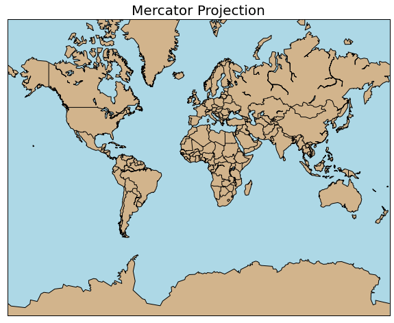
Create a global map with a Cylindrical Equidistant Projection
fig = plt.figure(figsize = (10,8))
m = Basemap(projection='cyl',llcrnrlat=-80,urcrnrlat=80,llcrnrlon=-180,urcrnrlon=180)
m.drawcoastlines()
m.fillcontinents(color='tan',lake_color='lightblue')
m.drawcountries(linewidth=1, linestyle='solid', color='k' )
m.drawmapboundary(fill_color='lightblue')
plt.title(" Cylindrical Equidistant Projection", fontsize=20)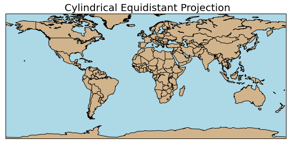
Create a global map with Orthographic Projection
fig = plt.figure(figsize = (10,8))
m = Basemap(projection='ortho', lon_0 = 25, lat_0 = 10)
m.drawcoastlines()
m.fillcontinents(color='tan',lake_color='lightblue')
m.drawcountries(linewidth=1, linestyle='solid', color='k' )
m.drawmapboundary(fill_color='lightblue')
plt.title("Orthographic Projection", fontsize=18)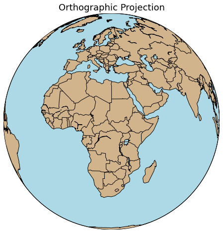
Create a global map with a Robinson Projection
fig = plt.figure(figsize = (10,8))
m = Basemap(projection='robin',llcrnrlat=-80,urcrnrlat=80,llcrnrlon=-180,urcrnrlon=180, lon_0 = 0, lat_0 = 0)
m.drawcoastlines()
m.fillcontinents(color='tan',lake_color='lightblue')
m.drawcountries(linewidth=1, linestyle='solid', color='k' )
m.drawmapboundary(fill_color='lightblue')
plt.title(" Robinson Projection", fontsize=20)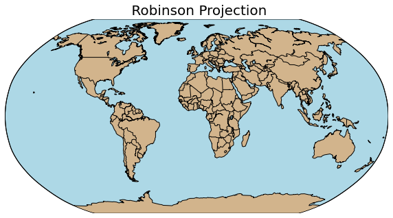
Plotting a specific region
a) By passing bounding box information (llcrnrlon, llcrnrlat, urcrnrlon,urcrnrlat)
fig = plt.figure(figsize = (10,8))
m = Basemap(projection='cyl',llcrnrlon=32.5,llcrnrlat=3,urcrnrlon=49,urcrnrlat=15, resolution = 'h')
m.drawcoastlines()
m.fillcontinents(color='tan',lake_color='lightblue')
m.drawcountries(linewidth=1, linestyle='solid', color='k' )
m.drawmapboundary(fill_color='lightblue')
m.drawcoastlines()
plt.show()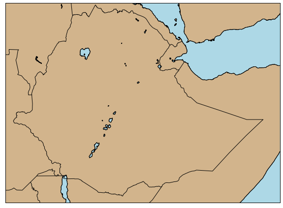
b) By passing the central longitude & central latitude, as well as the width, & height values.
Here, the width and height are given in meters.
fig = plt.figure(num=None, figsize=(12, 8) )
m = Basemap(projection='aea', width=1700000, height=1500000, resolution='h',lon_0= 40.5,lat_0=8.7)
m.fillcontinents(color='tan',lake_color='aqua')
m.drawmapboundary(fill_color='lightblue')
m.drawcountries(linewidth=1, linestyle='solid', color='k' )
m.drawcoastlines()
plt.show()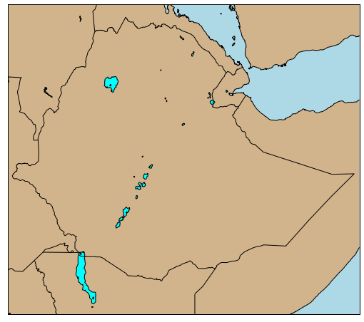
c) Make a regional map using the EPSG projection code
To find out more about the EPSG projection code, visit spatialreference.org
fig = plt.figure(figsize = (10,8))
m = Basemap(llcrnrlon=32.5,llcrnrlat=3,urcrnrlon=48.5, urcrnrlat=15, lat_0=7, lon_0 =37, resolution = 'l')
m.drawcoastlines()
m.fillcontinents(color='tan',lake_color='lightblue')
m.drawcountries(linewidth=1, linestyle='solid', color='k' )
m.drawmapboundary(fill_color='lightblue')
plt.title("Make a regional map using the EPSG projection code", fontsize=18)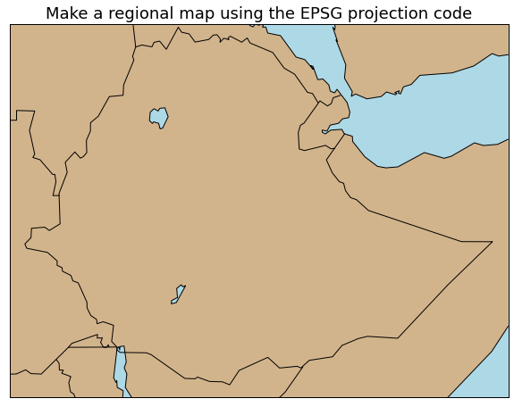
Let’s see how the resolution argument affects coastlines, lakes, country boundary lines
The available options are:
- c: crude
- l: low
- i: intermediate
- h: high
- f: full
fig = plt.figure(figsize = (16,16))

ax1 = plt.subplot2grid((3,2), (0,0))
ax2 = plt.subplot2grid((3,2), (0,1))
ax3 = plt.subplot2grid((3,2), (1,0))
ax4 = plt.subplot2grid((3,2), (1,1))

m1 = Basemap(llcrnrlon=32.5,llcrnrlat=3,urcrnrlon=48.5, urcrnrlat=15, ax=ax1, resolution = 'c')
m1.drawcoastlines()
m1.fillcontinents(color='tan',lake_color='lightblue')
m1.drawcountries(linewidth=1, linestyle='solid', color='k' )
m1.drawmapboundary(fill_color='lightblue')
plt.title("Crude resolution", fontsize=18)
ax1.set_title("Crude resolution", fontsize=18)

m2 = Basemap(llcrnrlon=32.5,llcrnrlat=3,urcrnrlon=48.5, urcrnrlat=15, ax=ax2, resolution = 'l')
m2.drawcoastlines()
m2.fillcontinents(color='tan',lake_color='lightblue')
m2.drawcountries(linewidth=1, linestyle='solid', color='k' )
m2.drawmapboundary(fill_color='lightblue')
ax2.set_title("Low resolution", fontsize=18)

m3 = Basemap(llcrnrlon=32.5,llcrnrlat=3,urcrnrlon=48.5, urcrnrlat=15, ax=ax3, resolution = 'i')
m3.drawcoastlines()
m3.fillcontinents(color='tan',lake_color='lightblue')
m3.drawcountries(linewidth=1, linestyle='solid', color='k' )
m3.drawmapboundary(fill_color='lightblue')
ax3.set_title("Intermediate resolution", fontsize=18)

m4 = Basemap(llcrnrlon=32.5,llcrnrlat=3,urcrnrlon=48.5, urcrnrlat=15, ax=ax4, resolution = 'h')
m4.drawcoastlines()
m4.fillcontinents(color='tan',lake_color='lightblue')
m4.drawcountries(linewidth=1, linestyle='solid', color='k' )
m4.drawmapboundary(fill_color='lightblue')
ax4.set_title("High resolution", fontsize=18)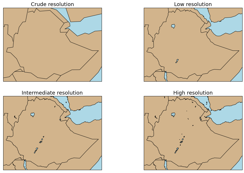
Background relief maps
Basemap provides several background relief images including:
a) Land-sea mask image
b) NASA blue marble
c) NOAA etopo
d) Shaded relief
a) Draw land-sea mask image
The
drawlsmask()function used to drawlakes,land, &oceansat onceIt avoids
fillcontinents&drawmapboundaryfunctionsThe
drawlsmask()function can take the following arguments:land_color: sets the color of the land (by default it’s gray)ocean_color: sets the color of the oceans (by default it’s white)resolution: sets the coastline resolution (by default it’s l, you can change it to: c, l, i , h, or f )lakes: plots lakes & ponds (by it default it’s True)grid: sets the land/sea mask grid spacing in minutes (by default it’s 5; You can change it to: 10, 2.5, & 1.25)
fig = plt.figure(figsize = (10,8))
m = Basemap(projection='cyl',llcrnrlon=32.5,llcrnrlat=3,urcrnrlon=49,urcrnrlat=15, resolution = 'i')
m.drawlsmask(land_color = "#ddaa66", ocean_color="#7777ff", resolution = 'i', lakes=True, grid=1.25)
m.drawcountries(linewidth=1, linestyle='solid', color='k' )
plt.title("Land-sea mask image", fontsize=20)
plt.show()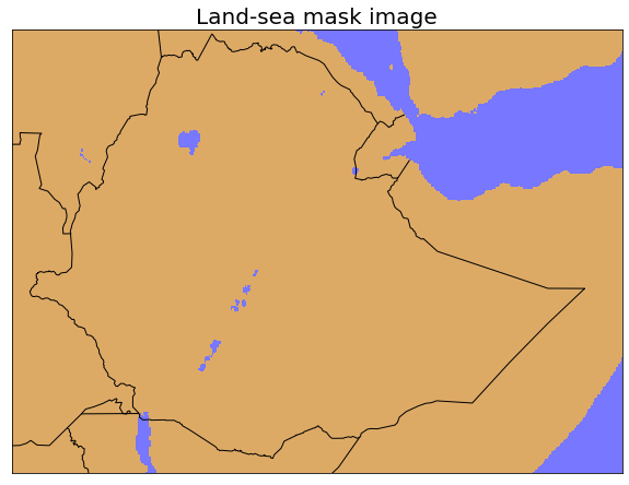
b) NASA Blue Marble image
- Use the
bluemarble()argument to apply the NASA blue marble image as a background map - To downgrade or upgrade image resolution use the scale argument
fig = plt.figure(figsize = (10,8))
m = Basemap(projection='cyl',llcrnrlon=32.5,llcrnrlat=3,urcrnrlon=49,urcrnrlat=15, resolution='i')
m.bluemarble(scale=1.0)
m.drawcoastlines()
m.drawcountries(linewidth=1, linestyle='solid', color='k' )
plt.title("NASA Blue Marble image as background map", fontsize=18)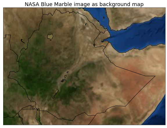
c) Shaded relief image
Use shadedrelief() argument to apply shaded relief image as a background map
fig = plt.figure(figsize = (10,8))
m = Basemap(projection='cyl',llcrnrlon=32.5,llcrnrlat=3,urcrnrlon=49,urcrnrlat=15, resolution='i')
m.shadedrelief()
m.drawcoastlines()
m.drawcountries(linewidth=1, linestyle='solid', color='k' )
plt.title("Shaded relief image as background map", fontsize=18)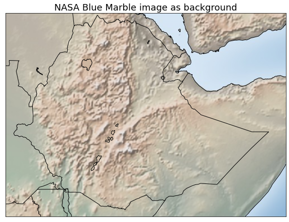
d) NOAAetopo relief image
Use etopo() argument to apply shaded relief image as a background map
fig = plt.figure(figsize = (10,8))
m = Basemap(projection='cyl',llcrnrlon=32.5,llcrnrlat=3,urcrnrlon=49,urcrnrlat=15, resolution='i')
m.etopo(scale=1.2)
m.drawcoastlines()
m.drawcountries(linewidth=1, linestyle='solid', color='k' )
plt.title("Shaded relief image as background map", fontsize=18)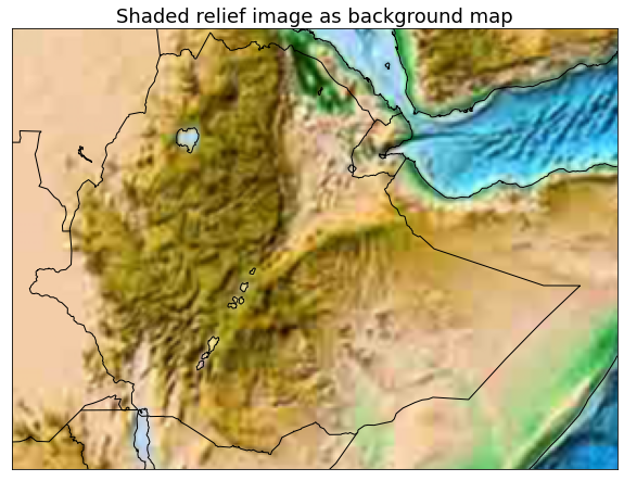
Plotting netCDF data using Basemap
Reading ECMWF temperature data
To read the netcdf data, we’ll use the Dataset class from the netcdf4-python library
from netCDF4 import Dataset as datasetThe netCDF data used in this tutorial have been saved at this URL. The netCDF file has 2-meter air temperature reanalysis data for the entire globe.
nc = dataset('.../ECMWF_temp2m.nc')Let’s read the coordinate variables (latitude, longitude, & time) & data variable (2-meter temperature) of the netCDF file.
lat = nc.variables['latitude'][:]
lon = nc.variables['longitude'][:]
time = nc.variables['time'][:]
t2 = nc.variables['p2t'][:]
Plotting filled contour maps:
Use the
contourf()function to draw filled contour mapsCreate a 2D
meshgridmatrix from 1D longitude & latitude arraysThe
contourf()function mainly takes:- longitude & latitude arrays
- data
- colormap
- levels
fig = plt.figure(num=None, figsize=(7, 7) )

m = Basemap(projection='cyl', llcrnrlon=32.5, llcrnrlat=3, urcrnrlon=49, urcrnrlat=15, resolution='i')
x, y = m(*np.meshgrid(lon,lat))

cs = m.contourf(x, y ,np.squeeze(t2[4,:,:]), levels = 100, cmap=plt.cm.jet)

m.drawcoastlines()
m.drawmapboundary()
m.drawcountries(linewidth=1, linestyle='solid', color='k' )

m.drawmeridians(range(33, 48, 2), color='k', linewidth=1.0, dashes=[4, 4], labels=[0, 0, 0, 1])
m.drawparallels(range(3, 15, 2), color='k', linewidth=1.0, dashes=[4, 4], labels=[1, 0, 0, 0])

plt.ylabel("Latitude", fontsize=15, labelpad=35)
plt.xlabel("Longitude", fontsize=15, labelpad=20)

cbar = m.colorbar(cs, location='right', pad="3%")
cbar.set_label('Temperature (K)', fontsize=13)

plt.title('2-meter temperature filled contour map', fontsize=15)
plt.show()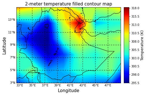
Plotting contour maps:
Use the
contour()function to draw contour mapsThe
contour()function uses similar arguments likecontourf()
fig = plt.figure(num=None, figsize=(7, 7))

m = Basemap(projection='cyl', llcrnrlon=32.5, llcrnrlat=3, urcrnrlon=49, urcrnrlat=15, resolution='i')
x, y = m(*np.meshgrid(lon,lat))

cs = m.contour(x, y ,np.squeeze(t2[4,:,:]), levels = 25 ,cmap=plt.cm.jet)

m.drawcoastlines()
m.drawmapboundary()
m.drawcountries(linewidth=1, linestyle='solid', color='k' )

m.drawmeridians(range(33, 48, 2), color='k', linewidth=1.0, dashes=[4, 4], labels=[0, 0, 0, 1])
m.drawparallels(range(3, 15, 2), color='k', linewidth=1.0, dashes=[4, 4], labels=[1, 0, 0, 0])

plt.ylabel("Latitude", fontsize=15, labelpad=35)
plt.xlabel("Longitude", fontsize=15, labelpad=20)

cbar = m.colorbar(cs, location='right', pad="3%")
cbar.set_label('Temperature (K)', fontsize=13)

plt.clabel(cs, inline=True, fmt='%1.0f', fontsize=12, colors='k')
plt.title('2-meter temperature contour map', fontsize=15)
plt.show()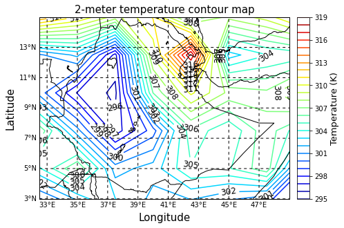
Plotting pseudo color maps:
- Use the
pcolor()orpcolormesh()function to draw pseudo color maps
fig = plt.figure(figsize=(7, 7) )

m = Basemap(projection='cyl', llcrnrlon=32.5, llcrnrlat=3, urcrnrlon=49, urcrnrlat=15, resolution='i')

cs = m.pcolor(x, y ,np.squeeze(t2[4,:,:]))
cs = m.pcolormesh(x, y ,np.squeeze(t2[4,:,:]))

pcolor(): draw a pseudocolor plot.
# pcolormesh(): draw a pseudocolor plot (faster version for regular meshes).

m.drawmeridians(range(33, 48, 2), color='k', linewidth=1.0, dashes=[4, 4], labels=[0, 0, 0, 1])
m.drawparallels(range(3, 15, 2), color='k', linewidth=1.0, dashes=[4, 4], labels=[1, 0, 0, 0])

m.drawcoastlines()
m.drawmapboundary()
m.drawcountries(linewidth=1, linestyle='solid', color='k' )

plt.ylabel("Latitude", fontsize=15, labelpad=35)
plt.xlabel("Longitude", fontsize=15, labelpad=20)

cbar = m.colorbar(cs, location='right', pad="3%")
cbar.set_label('Temperature (K)', fontsize=13)

plt.title('2-meter temperature pseudo-color map', fontsize=15)
plt.show()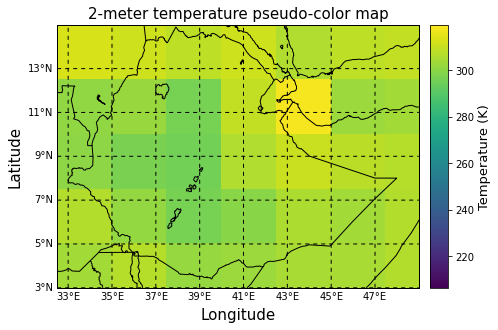
Well done! 🥇🥇🥇
I hope this tutorial has taught you the basics of Basemap plotting; if you found it useful, please leave your feedback in the comments!
Leave a Comment