Python Geopandas package for shapefile management

- Installing Geopandas package:
- Shapefile plotting
- Overlaying shapefiles
- Shapefile re-projectioning
- Shapefile Dissolving
- Shapefile clipping
- Exporting shapefile
Installing Geopandas package:
To start, add a new environment variable named geopandas_stable. Start ubuntu terminal & enter the following commands:
conda create --name geopandas_stable
Activate the geopandas_stable environment:
conda activate geopandas_stable
Add & set conda-forge channel:
  conda config --env --add channels conda-forge
  conda config --env --set channel_priority strict
Install Geopandas package with python-3:
conda install python=3 geopandas
Import the Geopandas library:
import geopandas as gpd
Check the Geopandas version:
print(gpd.__version__)
You have successfully installed Geopandas if you receive the version number. Finally, for reading & writing shapefiles, you can use any Python Notebook or IDE, such as Jupyter-Notebook & Spyder.
Reading & manipulating shapefile dataframes
Import the matplotlib library for visualization purposes:
  import matplotlib.pyplot as plt
  from matplotlib.ticker import ScalarFormatter
All of the shapefiles used in this tutorial have been compressed & saved at this URL
There are two methods to read the data:
- You can download the compressed shapefiles from the above link to your local directory, extract it, & use this local directory to locate the path of the shapefiles
- Or you can directly read the compressed shapefiles from the above site if you are connected to internate
Load the shapefile using gpd.read_file function:
  zipfile_basins = "https://yonsci.github.io/yon_academic//files/Geopandas_data/ETH_basins.zip"
  ET_basin = gpd.read_file(zipfile_basins)
Inspect the attribute table of the data by typing:
ET_basin
| AREA | PERIMETER | RIVERBASIN | RIVERBAS_1 | BASINNAME | layer | Basin_type | geometry | |
|---|---|---|---|---|---|---|---|---|
| 0 | 2.000141e+11 | 2836371.545 | 5 | 4 | ABBAY | Abby | 1 | POLYGON ((35.75669 12.67180, 35.75921 12.67317... |
| 1 | 1.121677e+11 | 2050391.912 | 6 | 5 | AWASH | Awash | 1 | POLYGON ((39.52930 11.72403, 39.52891 11.72624... |
| 2 | 4.755561e+09 | 318650.138 | 7 | 6 | AYSHA | Aysha | 1 | POLYGON ((42.30811 10.99144, 42.32126 10.99586... |
| 3 | 7.572123e+10 | 2128499.780 | 8 | 7 | BARO AKOBO | Baro_akobo | 1 | POLYGON ((34.47938 10.83318, 34.48112 10.83473... |
| 4 | 6.524619e+10 | 1228197.473 | 4 | 3 | DENAKIL | Denakil | 1 | POLYGON ((39.37495 14.50856, 39.41100 14.52892... |
| 5 | 1.722588e+11 | 2006366.812 | 13 | 12 | GENALE DAWA | Genale_dawa1 | 1 | POLYGON ((41.13743 6.94134, 41.14177 6.93580, ... |
| 6 | 5.868187e+09 | 534670.622 | 2 | 1 | MEREB GASH | Mereb1 | 1 | POLYGON ((37.80309 14.70250, 37.91271 14.88540... |
| 7 | 7.969898e+10 | 1613036.102 | 9 | 8 | OGADEN | Ogaden | 1 | POLYGON ((43.31527 9.60498, 43.35539 9.58202, ... |
| 8 | 7.871230e+10 | 1832234.370 | 11 | 10 | OMO GIBE | Omo_gibe | 1 | POLYGON ((38.02335 8.93136, 38.03574 8.91034, ... |
| 9 | 5.298484e+10 | 1381422.016 | 12 | 11 | RIFT VALLY | Rift_valley | 1 | POLYGON ((38.40912 8.39296, 38.41411 8.39297, ... |
| 10 | 8.367317e+10 | 1468016.695 | 3 | 2 | TEKEZE | Tekeze | 1 | POLYGON ((39.40391 14.25409, 39.45916 14.23977... |
| 11 | 2.017996e+11 | 2336905.978 | 10 | 9 | WABI SHEBELE | Wabi_shebelle | 1 | POLYGON ((42.69533 9.58651, 42.69804 9.58040, ... |
Instead of displaying the entire dataframe, I recommend displaying only the first & last 5 rows of the dataframe using the .head() & .tail() built-in functions. To display the first 5 rows of the dataframe, type:
ET_basin.head()
| AREA | PERIMETER | RIVERBASIN | RIVERBAS_1 | BASINNAME | layer | Basin_type | geometry | |
|---|---|---|---|---|---|---|---|---|
| 0 | 2.000141e+11 | 2836371.545 | 5 | 4 | ABBAY | Abby | 1 | POLYGON ((35.75669 12.67180, 35.75921 12.67317... |
| 1 | 1.121677e+11 | 2050391.912 | 6 | 5 | AWASH | Awash | 1 | POLYGON ((39.52930 11.72403, 39.52891 11.72624... |
| 2 | 4.755561e+09 | 318650.138 | 7 | 6 | AYSHA | Aysha | 1 | POLYGON ((42.30811 10.99144, 42.32126 10.99586... |
| 3 | 7.572123e+10 | 2128499.780 | 8 | 7 | BARO AKOBO | Baro_akobo | 1 | POLYGON ((34.47938 10.83318, 34.48112 10.83473... |
| 4 | 6.524619e+10 | 1228197.473 | 4 | 3 | DENAKIL | Denakil | 1 | POLYGON ((39.37495 14.50856, 39.41100 14.52892... |
Similarly, to display the last 5 rows of the dataframe, type:
ET_basin.tail()
| AREA | PERIMETER | RIVERBASIN | RIVERBAS_1 | BASINNAME | layer | Basin_type | geometry | |
|---|---|---|---|---|---|---|---|---|
| 7 | 7.969898e+10 | 1613036.102 | 9 | 8 | OGADEN | Ogaden | 1 | POLYGON ((43.31527 9.60498, 43.35539 9.58202, ... |
| 8 | 7.871230e+10 | 1832234.370 | 11 | 10 | OMO GIBE | Omo_gibe | 1 | POLYGON ((38.02335 8.93136, 38.03574 8.91034, ... |
| 9 | 5.298484e+10 | 1381422.016 | 12 | 11 | RIFT VALLY | Rift_valley | 1 | POLYGON ((38.40912 8.39296, 38.41411 8.39297, ... |
| 10 | 8.367317e+10 | 1468016.695 | 3 | 2 | TEKEZE | Tekeze | 1 | POLYGON ((39.40391 14.25409, 39.45916 14.23977... |
| 11 | 2.017996e+11 | 2336905.978 | 10 | 9 | WABI SHEBELE | Wabi_shebelle | 1 | POLYGON ((42.69533 9.58651, 42.69804 9.58040, ... |
Alternatively, you can view a specific section of the dataframe by defining the row numbers, but keep in mind that Python counts starting from zero. For example, to display only the 3rd & 4th rows, you can type:
ET_basin[3:5]
| AREA | PERIMETER | RIVERBASIN | RIVERBAS_1 | BASINNAME | layer | Basin_type | geometry | |
|---|---|---|---|---|---|---|---|---|
| 3 | 7.572123e+10 | 2128499.780 | 8 | 7 | BARO AKOBO | Baro_akobo | 1 | POLYGON ((34.47938 10.83318, 34.48112 10.83473... |
| 4 | 6.524619e+10 | 1228197.473 | 4 | 3 | DENAKIL | Denakil | 1 | POLYGON ((39.37495 14.50856, 39.41100 14.52892... |
To find out the size of the dataframe, type:
ET_basin.shape
Output: (12, 8)
As can be seen, the dataframe has 12 rows and 8 columns
To obtain the row numbers or length of the dataframe, type:
len(ET_basin)
Output: 12
To print the column names, type:
ET_basin.columns
Index(['AREA', 'PERIMETER', 'RIVERBASIN', 'RIVERBAS_1', 'BASINNAME', 'layer', 'Basin_type', 'geometry'], dtype='object')
To list the column’s contents:
ET_basin.BASINNAME.values
array(['ABBAY', 'AWASH', 'AYSHA', 'BARO AKOBO', 'DENAKIL', 'GENALE DAWA', 'MEREB GASH', 'OGADEN', 'OMO GIBE', 'RIFT VALLY', 'TEKEZE', 'WABI SHEBELE'], dtype=object)
To know how the data is represented or stored in the dataframe, type:
type(ET_basin)
geopandas.geodataframe.GeoDataFrame In this example, each vector data is represented as GeoDataFrame
The geometry column is the most essential of the columns & it contains the x-y coordinate values of the vector data. For instance, you can look at the values using .geometry function:
print(ET_basin.geometry)
0     POLYGON ((35.75669 12.67180, 35.75921 12.67317...
1     POLYGON ((39.52930 11.72403, 39.52891 11.72624...
2     POLYGON ((42.30811 10.99144, 42.32126 10.99586...
3     POLYGON ((34.47938 10.83318, 34.48112 10.83473...
4     POLYGON ((39.37495 14.50856, 39.41100 14.52892...
5     POLYGON ((41.13743 6.94134, 41.14177 6.93580, ...
6     POLYGON ((37.80309 14.70250, 37.91271 14.88540...
7     POLYGON ((43.31527 9.60498, 43.35539 9.58202, ...
8     POLYGON ((38.02335 8.93136, 38.03574 8.91034, ...
9     POLYGON ((38.40912 8.39296, 38.41411 8.39297, ...
10    POLYGON ((39.40391 14.25409, 39.45916 14.23977...
11    POLYGON ((42.69533 9.58651, 42.69804 9.58040, ...
Name: geometry, dtype: geometry
You can use the following function to extract x-y coordinate values of a given polygon, In this case, the first polygon:
  def coord_lister(geom):
  coords = list(geom.exterior.coords)
  return(coords)
  coordinates = ET_basin.geometry.apply(coord_lister)
  Abbay_coord = coordinates[0]
Let’s look at the first ten x-y coordinate values of the first polygon:
Abbay_coord[:10]
[(35.756690888078126, 12.671797097608444),
 (35.75921179031758, 12.673172165175462),
 (35.76174531616754, 12.674460456844615),
 (35.7643064966319, 12.675563955460834),
 (35.76690347742137, 12.676383429901467),
 (35.76954908459146, 12.676824219629998),
 (35.77224026615727, 12.676922403038853),
 (35.774962412059814, 12.676764711775403),
 (35.77771230490099, 12.676412056011529),
 (35.780480076318945, 12.675917364792335)]`
You can use the geom type function to get information about the geometry type (polygon, line, or point) of each data recorded in the dataframe:
ET_basin.geom_type
0     Polygon
1     Polygon
2     Polygon
3     Polygon
4     Polygon
5     Polygon
6     Polygon
7     Polygon
8     Polygon
9     Polygon
10    Polygon
11    Polygon
dtype: object As you can see, all of the vector types in the dataframe are polygons.
To view the spatial extent or coverage of the shapefile, use the total_bounds function:
ET_basin.total_bounds
array([33.00541327, 3.40510906, 47.99567693, 14.88539753])
The shapefile ranges from 33.00541327 to 47.99567693 longitudes & 3.40510906 to 14.88539753 latitudes
You may get a quick overview of the shape file by using the geometry values. For instance, to view the first data, you can use the code below:
ET_basin.at[0,'geometry']

Shapefile plotting
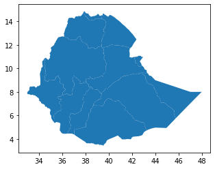
Let’s now make a simple plot of the shapefile using plot() function:
ET_basin.plot()
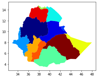
Let’s colorize the map with the cmap function:
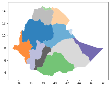
ET_basin.plot(cmap ='jet')
In place of jet, you can use one of the Matplotlib color options given below, or you can visit the following link to learn more about the colormaps:
'Accent', 'Accent_r', 'Blues', 'Blues_r', 'BrBG', 'BrBG_r', 'BuGn', 'BuGn_r', 'BuPu', 'BuPu_r', 'CMRmap', 'CMRmap_r', 'Dark2', 'Dark2_r', 'GnBu', 'GnBu_r', 'Greens', 'Greens_r', 'Greys', 'Greys_r', 'OrRd', 'OrRd_r', 'Oranges', 'Oranges_r', 'PRGn', 'PRGn_r', 'Paired', 'Paired_r', 'Pastel1', 'Pastel1_r', 'Pastel2', 'Pastel2_r', 'PiYG', 'PiYG_r', 'PuBu', 'PuBuGn', 'PuBuGn_r', 'PuBu_r', 'PuOr', 'PuOr_r', 'PuRd', 'PuRd_r', 'Purples', 'Purples_r', 'RdBu', 'RdBu_r', 'RdGy', 'RdGy_r', 'RdPu', 'RdPu_r', 'RdYlBu', 'RdYlBu_r', 'RdYlGn', 'RdYlGn_r', 'Reds', 'Reds_r', 'Set1', 'Set1_r', 'Set2', 'Set2_r', 'Set3', 'Set3_r', 'Spectral', 'Spectral_r', 'Wistia', 'Wistia_r', 'YlGn', 'YlGnBu', 'YlGnBu_r', 'YlGn_r', 'YlOrBr', 'YlOrBr_r', 'YlOrRd', 'YlOrRd_r', 'afmhot', 'afmhot_r', 'autumn', 'autumn_r', 'binary', 'binary_r', 'bone', 'bone_r', 'brg', 'brg_r', 'bwr', 'bwr_r', 'cividis', 'cividis_r', 'cool', 'cool_r', 'coolwarm', 'coolwarm_r', 'copper', 'copper_r', 'cubehelix', 'cubehelix_r', 'flag', 'flag_r', 'gist_earth', 'gist_earth_r', 'gist_gray', 'gist_gray_r', 'gist_heat', 'gist_heat_r', 'gist_ncar', 'gist_ncar_r', 'gist_rainbow', 'gist_rainbow_r', 'gist_stern', 'gist_stern_r', 'gist_yarg', 'gist_yarg_r', 'gnuplot', 'gnuplot2', 'gnuplot2_r', 'gnuplot_r', 'gray', 'gray_r', 'hot', 'hot_r', 'hsv', 'hsv_r', 'inferno', 'inferno_r', 'jet', 'jet_r', 'magma', 'magma_r', 'nipy_spectral', 'nipy_spectral_r', 'ocean', 'ocean_r', 'pink', 'pink_r', 'plasma', 'plasma_r', 'prism', 'prism_r', 'rainbow', 'rainbow_r', 'seismic', 'seismic_r', 'spring', 'spring_r', 'summer', 'summer_r', 'tab10', 'tab10_r', 'tab20', 'tab20_r', 'tab20b', 'tab20b_r', 'tab20c', 'tab20c_r', 'terrain', 'terrain_r', 'turbo', 'turbo_r', 'twilight', 'twilight_r', 'twilight_shifted', 'twilight_shifted_r', 'viridis', 'viridis_r', 'winter', 'winter_r'
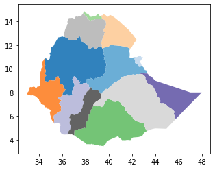
You can colorize the map based on a specific column, in this case, let’s use the BASINNAME column:
ET_basin.plot(cmap ='tab20c', column='BASINNAME')
You can also use the figsize option to change the plot size:
ET_basin.plot(cmap ='tab20c', column='BASINNAME', figsize=(6,6))
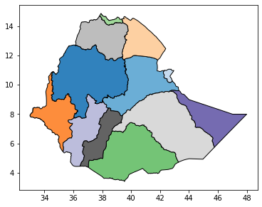
You can apply an edge color to each polygon in the shapefile using edgecolor function:
ET_basin.plot(cmap ='tab20c', column='BASINNAME', figsize=(6,6), edgecolor='black')
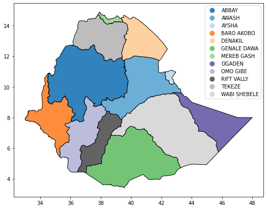
You may also put a legend in the plot:
ET_basin.plot(cmap ='tab20c', column='BASINNAME', figsize=(9,7), edgecolor='black', legend=True)
However, using the matplotlib functions is a more convenient way to make plots:
  fig, ax = plt.subplots(figsize=(9,7))
  ET_basin.plot(alpha=1.0, cmap ='tab20c', column='BASINNAME', edgecolor='black', legend=True, ax=ax )
  ax.set_title('Major river basins of Ethiopia', fontsize=25)
  ax.set_xlabel("Longitude (Degrees)", fontsize=12)
  plt.show()

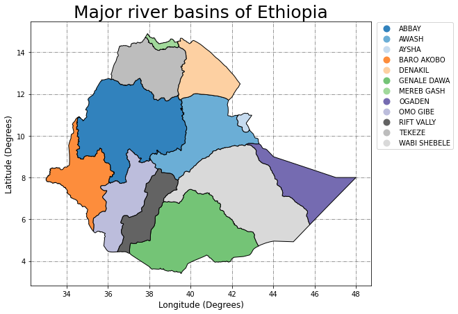
You can use the script underneath to add grids to the plot:
  fig, ax = plt.subplots(figsize=(9,7))
  ET_basin.plot(alpha=1.0, cmap ='tab20c', column='BASINNAME', edgecolor='black', legend=True, ax=ax )
  ax.set_title('Major river basins of Ethiopia', fontsize=25)
  ax.set_axisbelow(True)
  ax.yaxis.grid(color='gray', linestyle='dashdot')
  ax.xaxis.grid(color='gray', linestyle='dashdot')
  ax.set_xlabel("Longitude (Degrees)", fontsize=12)
  ax.set_ylabel("Latitude (Degrees)", fontsize=12)
  plt.show()
Here, instead of dashdot you can use dotted, dashed, solid 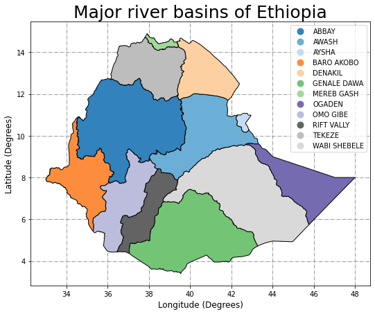
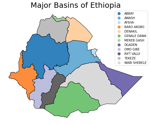
You can remove the grids & boundary lines by using the code below:
  fig, ax = plt.subplots(figsize=(9,7))
  ET_basin.plot(alpha=1.0, cmap ='tab20c', column='BASINNAME', edgecolor='black', legend=True, ax=ax )
  ax.set_title('Major Basins of Ethiopia', fontsize=25)
  ax.set_axis_off()
  plt.show()
You can also change the legend’s position:
  fig, ax = plt.subplots(figsize=(9,7))
  ET_basin.plot(alpha=1.0, cmap ='tab20c', column='BASINNAME', edgecolor='black', ax=ax, legend=True )
  ax.set_title('Major river basins of Ethiopia', fontsize=25)
  ax.set_axisbelow(True)
  ax.yaxis.grid(color='gray', linestyle='dashdot')
  ax.xaxis.grid(color='gray', linestyle='dashdot')
  ax.set_xlabel("Longitude (Degrees)", fontsize=12)
  ax.set_ylabel("Latitude (Degrees)", fontsize=12)
  leg = ax.get_legend()
  leg.set_bbox_to_anchor((1.25,1.01))
  plt.show()
Plots can be saved as image files using the plt. savefig() function:
  fig, ax = plt.subplots(figsize=(9,7))
  ET_basin.plot(alpha=1.0, cmap ='tab20c', column='BASINNAME', edgecolor='black', legend=True, ax=ax )
  ax.set_title('Major river basins of Ethiopia', fontsize=25)
  ax.set_axisbelow(True)
  ax.yaxis.grid(color='gray', linestyle='dashdot')
  ax.xaxis.grid(color='gray', linestyle='dashdot')
  ax.set_xlabel("Longitude (Degrees)", fontsize=12)
  ax.set_ylabel("Latitude (Degrees)", fontsize=12)
  plt.savefig('basins.jpeg', transparent=True,  bbox_inches='tight', dpi=800)
  plt.show()

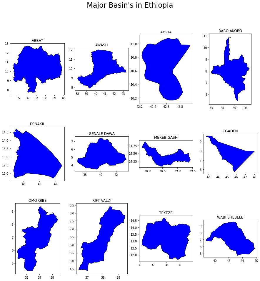
Making subplots:
fig, ((ax1, ax2, ax3, ax4), (ax5, ax6, ax7, ax8), (ax9, ax10, ax11, ax12)) = plt.subplots(3, 4, figsize=(15,15))
fig.suptitle("Major Basin's in Ethiopia", fontsize=24)
  ET_basin.loc[ET_basin.BASINNAME == "ABBAY"].plot(ax=ax1, facecolor='Blue',  edgecolor='black')
ax1.set_title("ABBAY")
  ET_basin.loc[ET_basin.BASINNAME == "AWASH"].plot(ax=ax2, facecolor='Blue',  edgecolor='black')
ax2.set_title("AWASH")
  ET_basin.loc[ET_basin.BASINNAME == "AYSHA"].plot(ax=ax3, facecolor='Blue',  edgecolor='black')
ax3.set_title("AYSHA")
  ET_basin.loc[ET_basin.BASINNAME == "BARO AKOBO"].plot(ax=ax4, facecolor='Blue',  edgecolor='black')
ax4.set_title("BARO AKOBO")
  ET_basin.loc[ET_basin.BASINNAME == "DENAKIL"].plot(ax=ax5, facecolor='Blue',  edgecolor='black')
ax5.set_title("DENAKIL")
  ET_basin.loc[ET_basin.BASINNAME == "GENALE DAWA"].plot(ax=ax6, facecolor='Blue',  edgecolor='black')
ax6.set_title("GENALE DAWA")
  ET_basin.loc[ET_basin.BASINNAME == "MEREB GASH"].plot(ax=ax7, facecolor='Blue',  edgecolor='black')
ax7.set_title("MEREB GASH")
  ET_basin.loc[ET_basin.BASINNAME == "OGADEN"].plot(ax=ax8, facecolor='Blue',  edgecolor='black')
ax8.set_title("OGADEN")
  ET_basin.loc[ET_basin.BASINNAME == "OMO GIBE"].plot(ax=ax9, facecolor='Blue',  edgecolor='black')
ax9.set_title("OMO GIBE")
  ET_basin.loc[ET_basin.BASINNAME == "RIFT VALLY"].plot(ax=ax10, facecolor='Blue',  edgecolor='black')
ax10.set_title("RIFT VALLY")
  ET_basin.loc[ET_basin.BASINNAME == "TEKEZE"].plot(ax=ax11, facecolor='Blue',  edgecolor='black')
ax11.set_title("TEKEZE")
  ET_basin.loc[ET_basin.BASINNAME == "WABI SHEBELE"].plot(ax=ax12, facecolor='Blue',  edgecolor='black')
ax12.set_title("WABI SHEBELE")
  plt.show()
Overlaying shapefiles
As an example, consider overlaying the ET_basin over the African continent shapefile, Let’s begin by importing the African continent shapefile:
  zipfile_Africa = "https://yonsci.github.io/yon_academic//files/Geopandas_data/Africa.zip"
  AFRICA = gpd.read_file(zipfile_Africa)
It is critical to remember that the coordinate systems of the two shapefiles must be identical. The .crs command can be used to verify the coordinate system of the two shapefiles:
AFRICA.crs
<Geographic 2D CRS: EPSG:4326>
Name: WGS 84
Axis Info [ellipsoidal]:
- Lat[north]: Geodetic latitude (degree)
- Lon[east]: Geodetic longitude (degree)
Area of Use:
- name: World
- bounds: (-180.0, -90.0, 180.0, 90.0)
Datum: World Geodetic System 1984
- Ellipsoid: WGS 84
- Prime Meridian: Greenwich
ET_basin.crs
<Geographic 2D CRS: EPSG:4326>
Name: WGS 84
Axis Info [ellipsoidal]:
- Lat[north]: Geodetic latitude (degree)
- Lon[east]: Geodetic longitude (degree)
Area of Use:
- name: World
- bounds: (-180.0, -90.0, 180.0, 90.0)
Datum: World Geodetic System 1984
- Ellipsoid: WGS 84
- Prime Meridian: Greenwich
You can see that they both use the WGS-84 geographic coordinate system (EPSG:4326)
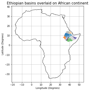
Now, you can plot the overlaid map using the following code:
  fig, ax = plt.subplots(figsize=(6,6))
  AFRICA.plot(ax=ax, color ='None', edgecolor='black')
  ET_basin.plot(ax=ax, cmap ='tab20c', column='BASINNAME')
  ax.grid(True)
  ax.set_title('Ethiopian basins overlaid on African continent', fontsize=15)
  ax.set(xlabel="Longitude (Degrees)", ylabel="Latitude (Degrees)")
  plt.show()
Shapefile re-projectioning
Some examples of widely used spatial reference systems:
| Reference systems name | EPSG code |
|---|---|
| WGS-84(Geographic) | EPSG:4326 |
| WGS_UTM_37N (projected) | EPSG:32637 |
| Spherical Mercator (projected) | EPSG:3857 |
| World Equidistant cylindrical/spherical | EPSG:4088 |
| World Equidistant cylindrical | EPSG:4087 |
| WGS84/ World Mercator | EPSG:3395 |
| WGS84/ World Pseudo Mercator | EPSG:3857 |
| World Robinson | EPSG:54030 |
If you need more information or want to access several reference coordinate systems, go to the following website.
Let’s re-project the ET_basin shapefile from WGS-84 geographic coordinate system to the Universal Transverse Mercator (UTM) projected coordinate system.
Re-projecting from EPSG:4326 to EPSG:32637:
  ET_basin_utm = ET_basin.to_crs({'init': 'epsg:32637'})
  Or simply type:
  ET_basin_utm = ET_basin.to_crs(32637)
Let’s review the coordinate system of the modified shapefile:
ET_basin_utm.crs
<Projected CRS: EPSG:32637>
Name: WGS 84 / UTM zone 37N
Axis Info [cartesian]:
- E[east]: Easting (metre)
- N[north]: Northing (metre)
Area of Use:
- name: World - N hemisphere - 36°E to 42°E - by country
- bounds: (36.0, 0.0, 42.0, 84.0)
Coordinate Operation:
- name: UTM zone 37N
- method: Transverse Mercator
Datum: World Geodetic System 1984
- Ellipsoid: WGS 84
- Prime Meridian: Greenwich
As you can see, it has been converted to the UTM projection.
You can also confirm by inspecting the shapefile boundaries:
ET_basin_utm.total_bounds
array([-161882.56221284, 376388.12499996, 1495282.8685069 , 1645935.62500012])
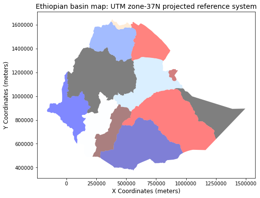
Let’s have a look at the new map under the projected UTM reference system:
  fig, ax = plt.subplots(figsize=(8, 8))
  ET_basin_utm.plot(cmap='flag_r', ax=ax, alpha=.5)
  ax.set_title("Ethiopian basin map: UTM zone-37N projected reference system", fontsize=14)
  ax.set_xlabel("X Coordinates (meters)", fontsize=12)
  ax.set_ylabel("Y Coordinates (meters)", fontsize=12)
  for axis in [ax.xaxis, ax.yaxis]:
  formatter = ScalarFormatter()
  formatter.set_scientific(False)
  axis.set_major_formatter(formatter)
You can also override the existing CRS of a given shapefile by using the .set_crs function:
ET_basin = ET_basin.set_crs(4088, allow_override=True)
Shapefile Dissolving
Dissolving polygon (removes the interior geometry). For example, let’s join the basin’s within the ET_basin shapefile to generate the Ethiopian boundary map. To do that, you need to pick which columns you want to maintain & the criteria for dissolving the shapefile.
In this example, the Basin_type will be used as a criteria & we want to maintain the geometry field only. To do this, use the code below:
ET_basin_selected = ET_basin[['Basin_type', 'geometry']]
Then, use the .dissolve() function, which works based on a unique attribute value
ET_dissolved = ET_basin_selected.dissolve(by='Basin_type')
Let’s view the resulting geodataframe:
ET_dissolved
| geometry | |
|---|---|
| Basin_type | |
| 1 | POLYGON ((43.28204 4.71709, 43.25243 4.70156, ... |
As you can see, the dataframe contains the geometry & Basin_type fields only.
Now we can plot & see the resulting boundary map:
ET_dissolved.plot()

Shapefile clipping
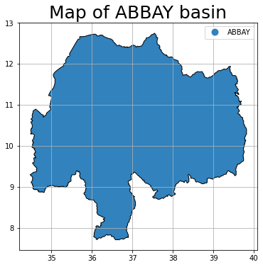
You may easily clip each polygon by selecting the desired column name & it’s unique value. In this situation, let’s use the BASINNAME as a column & (ABBAY) as a desired value from the ET_basin geodataframe.
To do that type the following:
Abbay_basin = ET_basin.loc[ET_basin.BASINNAME == "ABBAY"]
Now, let’s plot the clipped Abbay basin:
  fig, ax = plt.subplots(figsize=(6,6))
  Abbay_basin.plot(alpha=1.0, cmap ='tab20c', column='BASINNAME', edgecolor='black', legend=True, ax=ax )
  ax.set_title('Map of ABBAY basin', fontsize=25)
  ax.grid(True)
  plt.show()
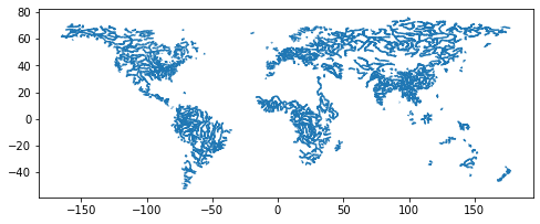
You can also use the intersection tool to clip data to a specified region, for instance, let’s load the major world river shapefile, & clip it to the Ethiopian region.
First, load the major world rivers:
  zip_World_river = "https://yonsci.github.io/yon_academic//files/Geopandas_data/world_rivers.zip"
  World_river = gpd.read_file(zip_World_river)
Let’s have a look at the loaded map:
World_river.plot(figsize=(8,8))
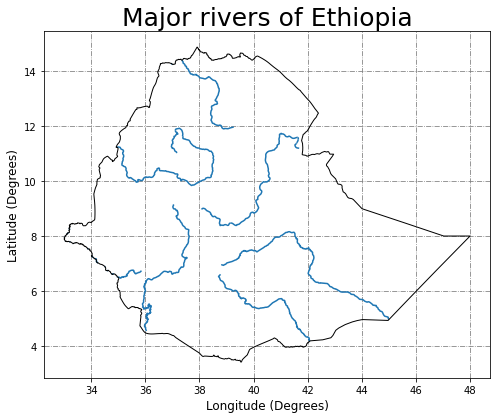
Let’s use the ET_dissolved shapefile to clip the world rivers to the area of interest:
Intersecting_rivers = gpd.overlay(ET_dissolved, World_river, how ='intersection', keep_geom_type=False)
Let’s plot the clipped major rivers over Ethiopia:
  fig, ax = plt.subplots(figsize=(8, 8))
  ET_dissolved.plot(alpha=1, facecolor="none", edgecolor="black", zorder=10, ax=ax)
  Intersecting_rivers.plot(ax=ax, legend=True)
  ax.yaxis.grid(color='gray', linestyle='dashdot')
  ax.xaxis.grid(color='gray', linestyle='dashdot')
  ax.set_xlabel("Longitude (Degrees)", fontsize=12)
  ax.set_ylabel("Latitude (Degrees)", fontsize=12)
  ax.set_title('Major rivers of Ethiopia', fontsize=25)
  plt.show()
Exporting shapefile
You can export the geopandas dataframe mailny to ESRI shapefile format (.shp) & GeoJSON (.json) file formats.
To export your geopandas dataframe as a shapefile:
ET_basin_utm.to_file("Basins_ethio.shp")
To export your geopandas dataframe as a GeoJSON file:
ET_basin_utm.to_file("ET_basin_utm_js.json", driver="GeoJSON")
Well done! 🥇🥇🥇 Good luck!
I hope this tutorial has given you the basics of geopandas package; if you find it useful in your work, please share your thoughts in the comments section!
Leave a Comment